LINEST Mystery output

[hAltonJones]

I have a small, simple table. I'm trying to do a simple multiple linear regression analysis. I get a single digit as a result. Here's the table and output. Here's the formula I used: =LINEST(D1:D10,A1:C10,TRUE,TRUE)

I fear the answer will be "You're an idiot", but that notwithstanding, what am I missing?

Thanks.

19.80          17.40     5.00      -48.00

17.50          15.60     5.10      -40.00

31.70          13.30     1.60      -39.00

19.90          14.70     1.70      -39.00

20.30          14.30     7.20      -36.00

20.60            1.60     1.70      -30.00

18.50          17.20    10.60     -24.00

20.90          14.00      7.80     -22.00

18.20          12.70    12.60     -21.00

19.30          14.30     0.10      -18.00

0.635946

[#2]

@hAltonJones 

It's not clear what you'd like to receive - where is x, where y, and why do you need regression stats array with last parameter. Please check if you are in sync with description LINEST function - Office Support (microsoft.com)

[#3]

@Sergei BaklanMy understanding (from the Help file) is that the first parameter is the "Y" column, i.e., the dependent variable, hence, LINEST(D1:D10,A1:C10,TRUE,TRUE). "X" variable, i.e., independent variables per the Help file are the second parameter, i.e., LINEST(D1:D10,A1:C10,TRUE,TRUE). In that I haven't received the results promised in the Help file, I don't know if I need the regression stats array, but I'm guessing it contains valuable information about the strength of the correlations, etc.

[#4]

@hAltonJones 

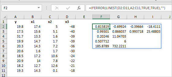
I see, thank you. Perhaps you are on Excel without dynamic arrays, in this case you shall use Ctrl+Shift+Enter, step by step tutorial for such is here Excel LINEST function with formula examples (ablebits.com) 

On modern Excel it looks like