Juggling items from one column to it's corresponding row in a new column

[Robert_Peltzman]

I've got an inventory list in column A of all my meds (about 300). I've got a medication usage list in a different column (say, C) that only has the list of meds that I've dispensed in the last month (about 90). If I can get each of the meds in the C column to appear on the same line as the corresponding drug in column A, I could easily subtract col. C from col. A to get my current inventory. Is there an easy way to do this without cutting and pasting each med from column C to it's correct line in a new column?

[#2]

@Robert_Peltzman  Hi,

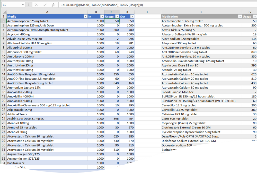
With Excel 365 you can  have cell B1
=XLOOKUP(A1;C:C;D:D;"")
being similar to in older versions of Excel, use
=IFERROR(VLOOKUP(A1;C:D;2;0);0)
and in both cases fill down or.

Even better, select in column A an Insert:table. Your formulas will then expand with the number of rows in the table.

Both columns Usage and Out are calculated.

Beware though that if you undo a change in a tables column formula, you may have to undo two or three times to come back to previous state.

[#3]

@Robert_Peltzman This would be something for VLOOKUP or XLOOKUP is your Excel version supports it. But, your data seems to be inconsistent. One med on the shorter list does not exist in the long list (marked yellow) and four meds on the short list seem to have different names (marked orange). For instance, "GlipiZIDE 10 mg tablet" vs. "Glipizide 10mg tablet". Either of the lookup functions will not match them. Then you have some double entries in the long list, also causing trouble. "Garbage in, garbage out".

I've reconciled the lists for you (using VLOOKUP as it works for all Excel versions), trusting that it will enable you to clean-up the data yourself. 

See attached file.

[#4]

Wow, thanks, I'll correct those errors and give it a try!
Robert

[#5]

Thanks Bos. This gives some options to play with.

[#6]

Before I try some of those formulas, tomorrow, I've got one more question: The meds in column C all have numbers associated with then in col. D (not shown). After I move col. C, over, how do I reattach those numbers to the items in the new Col. B?

[#7]

@Robert_Peltzman,

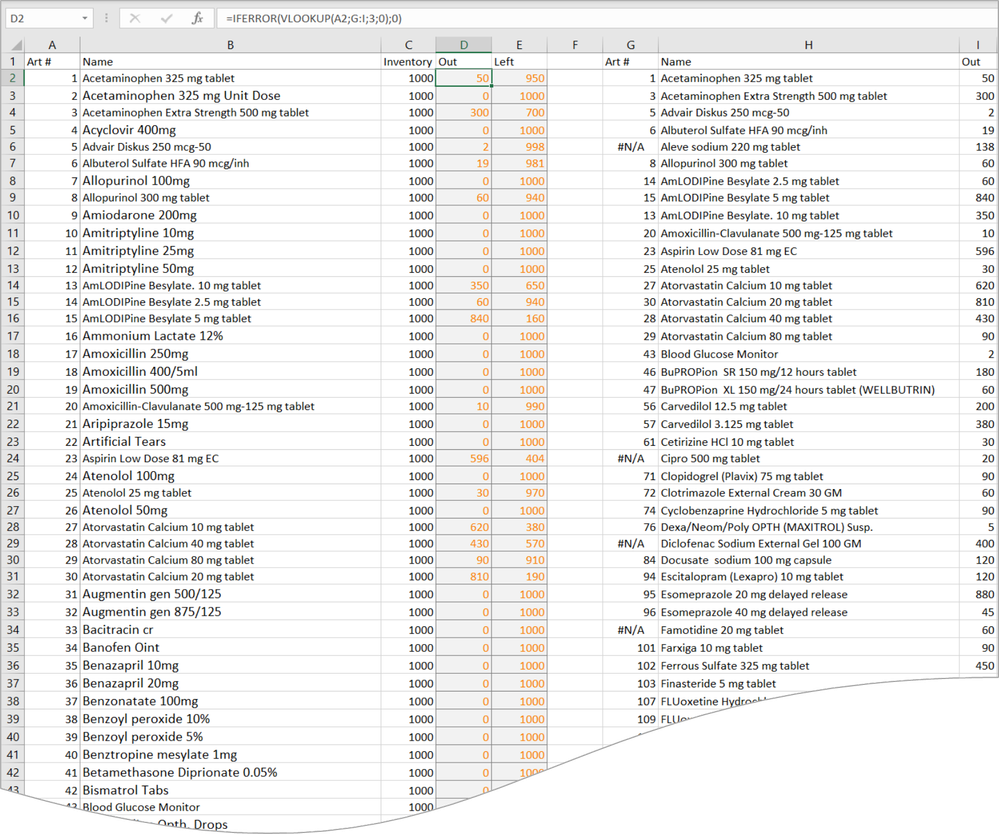
Mm... if you have the article numbers, use them instead of the names and you will get better results since it may happen that two different numbers share the same name.

Adjust the formulas to use the numbers;

D2    =IFERROR(VLOOKUP(A2;G:I;3;0);0)

[#8]

What I posted was just a small part of the spreadsheet, Darn, this looks better than my original.
Thank you!
I'm going to try that.

[#9]

:) You're welcome.
Also, by using the article numbers/ID's even in the shorter list you will cut the risk of misspelling the names and thus miss or point wrong in the inventory list.
If you continue using names in the subscription/small list (that may be what you are used to since it is more handy), it will be a good idea to append also Riny van Eekelens formulas to see that you get an inventory match on the name.

[#10]

My version of Excel doesn't like this formula =IFERROR(VLOOKUP(A2;G:I;3;0);0)
I've got Office Professional Plus 2019
Could that be the problem?

[#11]

Also, what does the 3 do, in the formula? I know 1 and 2 have to do with matching exactly or closely.

[#12]

@Robert_Peltzman 

I do not have the same national/local settings as you, and have semi colon where your version expects a comma.

Using the attached file should overcome that, or change ; to comma.

The parameter with 3 means column number three in the lookup area. It is though better to start using xlookup. It also has the parameter you refer to by default set to match exactly.

(there seems to be an issue with attaching files - let me know if you need it another way)

[#13]

Aha, that makes sense.