Join two spill ranges to one range with two columns

[mlylyly]

Hi community

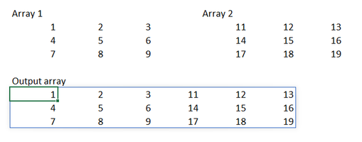
I would like to join two spill ranges into one range with two columns but cannot figure out how to do it. What I would like is the new range below. I believe it is what HSTACK() does but I do not have access to O365 yet through my corporate Excel. 

Any solution to this?

Thanks!

[#2 · Accepted solution]

@mlylyly 

For this task you can also use the CHOOSE() function in older Excel versions.

=CHOOSE({1,2},E4:E6,G4:G6)

In cases where your Range 1 = E4:E6 and Range 2 = G4:G6.

In older versions of Excel you have to finish this with CTRL + SHIFT + ENTER as an array formula.

[#3]

@mlylyly 

If you're looking to join two spills, then you most likely have 365 but without HSTACK (Possibly on Semi-Annual channel).  This might work in your version.

=IF({1,0},A1#,C1#)

[#4]

Thanks, I used dscheikey's version, worked like a charm!

[#5]

@Patrick2788 

@dscheikey 

Both of your solutions work but I have to expand it to joining to arrays with multiple columns, do you have a solution for that? 

I tried a simple expansion of both of your formulas but either seem to work.

Thanks in advance!

P.s., yes I have 365 but without HSTACK due to semi-annual channel, you're right

[#6]

@mlylyly 

You could do this:

=FILTER(A2:G4,A2:G2<>"")

[#7]

Thanks but I am looking for a solution which would work in a let() function without helper spills

[#8]

Where are the "helper spills" ?

[#9]

Maybe I'm not following but if I have a formula with

=LET(arrray1,array2,output) I cannot refer to ranges across the two arrays e.g., A2:G4 and A2:G2 which covers both array1 and array2

[#10]

@mlylyly 

Somewhat less elegant but playing with indices will work.

= LET(
      k, SEQUENCE(1,6),
      h, SEQUENCE(3),
      IF(k<4, array1#, INDEX(array2#,h,k-3))
   )

Of course, provided you have Lambda, you could always provide some window dressing

WorksheetFormula
= HStackλ(array1#, array2#)

HStackλ 
= LAMBDA(a₁, a₂,
     LET(
        k, SEQUENCE(1, COLUMNS(a₁) + COLUMNS(a₂)),
        h, SEQUENCE(MAX(ROWS(a₁), ROWS(a₂))),
        IF(k < 4, a₁, INDEX(a₂, h, k - 3))
     )
  )

Then again, you could make a case to corporate IT to put you on to the Insider beta channel so that you could preview new functionality on behalf of the company.

[#11]

@mlylyly 

If your real data is also as simple as the example, I would do it that way:

=LET(array1,A2#,array2,E2#,INDEX(array1:array2,{1;2;3},{1,2,3,5,6,7}))

[#12]

@mlylyly 

Try this:

=LET(dynamic,A2#:E2#,c,COLUMNS(dynamic),top,INDEX(dynamic,1,SEQUENCE(,c)),FILTER(dynamic,top<>0))

[#13]

What I was looking for, thanks a lot!