Insert the numbers of a table in the last row of a different table (no VB)

[MRAfshar3000]

Is there a formula that can put the numbers in a table in the last row of the different table? (no VB) 

[#2]

Hi @MRAfshar3000 

could you please provide an example of what you want to achieve? 

At least some screenshots would help.

[#3]

Consider that the mineral, gold, silver, copper, gypsum, coal and iron mining, and each storage die and fall into the pit. (At the top of each well is written which one it is for) Here is my table from which the information should be extracted and automatically placed in a different and relevant table, unlike the well that is poured the later, the higher the The table is lower. I have the column ABCD and the columns (A and B) are never filled in the same row, and so on (C and D), for example: I have A1 B2 and C1 D2, the word in A1 says Which table should C1 be in and B2 in the same way

[#4]

Hi @MRAfshar3000 

I'm sorry, but it's still confusing for me. Could you please upload an example of your file?

Or at least some screenshots where I could see which information should go where under which conditions. 

[#5]

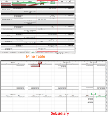
I tried to show my meaning in the photo

substations are not accurate , so I want to use the functions for entering numbers

@Martin_Weiss 

[#6 · Accepted solution]

Hi @MRAfshar3000 

thanks for the screenshots, this is much better. So, it looks like what we call T-accounts, where you put something on the debit side and something on the credit side.

There is probably an easy solution if you use Microsoft 365 / Office 365 (and Excel 2021), because there you have the new dynamic array functions like FILTER.

I tried to rebuild a small example, I have also attached the example file:

So in the above example, the formula in A14 would be:

=IFERROR(FILTER(A2:A8;C2:C8=A12);0)

The surrounding IFERROR just avoids that you get #KALK-errors if an account name is not found.

Just note, that depending on your regional local settings you might need to replace ; with ,

So 

=IFERROR(FILTER(A2:A8,C2:C8=A12),0)

The bad news is, that this FILTER-function is not available in older Excel versions before Excel 2021. In this case, I do not have a solution for you, unfortunately.

[#7]

I really thank you
You helped me a lot
Fortunately, my version is Minecraft 365
I think you are also an accountant, so if it is possible to say some terms, for example, the same main table, we say newspaper book (my country)
In private