Index removing duplicates

[Machala Sentance]

Hi

I think that there is a simple amendment to this but I have been going around in circles.  I have a large dataset and I need to be able to list all instances that something appears, I have the following formula that does what it should but I want it to be able to not return duplicate values, so for example there may be 2 groups with the same name but each has a different row due to the time an event takes place so I just need it to return this once (using the name):

{=INDEX($U$2:$U$986,SMALL(IF(Blank!$B$4=$S$2:$S$986,ROW(U$2:$U$986)-ROW($U$2)+1),ROW(1:1)))}

Thanks in advance

[#2]

@Machala Sentance 

I see you've had a lot of views to your question and no responses. If I might be bold here, it's partly, I suspect, because your question isn't exactly clear. It would help if you could post either the actual spreadsheet OR, if that contains confidential information, a mockup that illustrates the problem you're trying to solve.

All of that said, another approach to retrieving just one instance of a name or something that appears more than once, is the new UNIQUE function. Using it might resolve your issue. And if you specifically want to retrieve just one instance of the occurrence of the name "Michala" (for example) you could use FILTER in conjunction with UNIQUE.

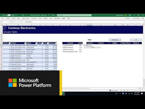
These do require the most recent version of Excel. From what you've written I am going to assume that you could write the formula on your own given some instruction, so here's an excellent introductory video on those new functions. https://www.youtube.com/watch?v=9I9DtFOVPIg

[#3]

@mathetes 

Thanks for the reply, I have watch this and unfortunatley does not given me what I am really wanting (maybe it's impossible :)).

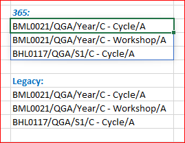
I have attached a mock up of part of the spreadsheet shwowing where and what I am trying to do - if this is still not clear please let me know.

I just need the activity to show once for the relevant staff member

Thanks again for all help

[#4]

@Machala Sentance 

Depends on your version of Excel

with

=UNIQUE(FILTER(Summary!C:C,Summary!B:B=C5))

or
=IFERROR(INDEX( Summary!$C$1:INDEX(Summary!C:C,COUNTA(Summary!C:C) ),
  AGGREGATE(15,6,1/
        ( Summary!$B$1:INDEX(Summary!B:B,COUNTA(Summary!C:C) ) =$C$5)/
        (COUNTIF($B$28:B28,  Summary!$C$1:INDEX(Summary!C:C,COUNTA(Summary!C:C) ) )=0)*
        ROW( Summary!$C$1:INDEX(Summary!C:C,COUNTA(Summary!C:C) )  ),1)),
 "")
and drag it down

[#5 · Accepted solution]

@Machala Sentance 

Check this. I think FILTER and UNIQUE does work
=UNIQUE(FILTER(Table1[Activity template hk],Table1[Suggested Staff hk]=C5,"None found"))

That's the formula I entered and it seemed to me at any rate that it produces the result you are looking for. I've attached the revised spreadsheet.

This first performs a FILTERing of the activity column based on the staff ID

Then the UNIQUE eliminates duplicates.

[#6]

@mathetes 

@Sergei Baklan 

Hi Both

Many thanks for the replies, both work perfectly

Apologies I couldn't get the Unique/Filter to work but I now have a better understanding of it.

Thanks again