Index match not working on 365 for mac

[Chris_Walsh]

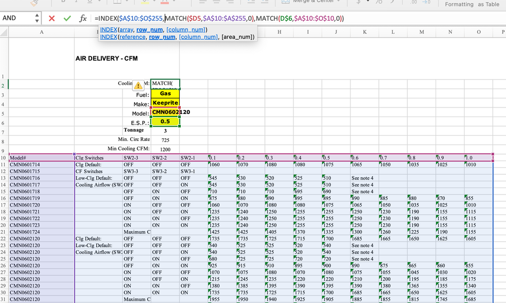
Trying to have index and match pick data from a table (but its not a “Table”): 

Index = table data F11: O255

 Match Reference 1 is D5 (this is a drop down list with values entered as reference in data validation, from a different part of the sheet) with Model numbers in column A11:A255

Match reference 2 is D6 (this is a drop down list with values entered in data validation separated by commas) with Headers on Row F10:O10

Match Reference 3 is D9 and must find 1st and Closest Match equal to or greater than D9

The formula i have been trying to get to work with not luck, is just to find the 1st match Using the first two match references D5 and D6 (see Image attached) i need this to work to but it returns a #N/A. This is after i trimmed and cleaned the data from the original table and copied the values to their current location… this trim clean did create duplicates however i will have duplicate numbers anyway which is why i want to find the 1st closets match equal to or grater than D9. All cells are formatted as “General”. 

Any help or advice would be greatly appreciated! I have been working on this equation for days and can’t figure it out. 

[#2]

@Chris_Walsh 

It's not totally clear what result you're expecting. My best guess, an inference from the INDEX portion of your formula, is that you're hoping to retrieve one entire row from the range $A$10:$O$255, whatever row meets the two criteria set up in the pair of MATCH functions. IF that is indeed the case, you will have better luck using the newer FILTER function, which also takes multiple criteria, which you are also attempting to implement.

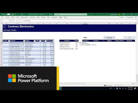
And lucky for you, since you are working with 365 on a Mac (as am I) you'll be able to use FILTER. Here's a link to an excellent introductory video Microsoft used to introduce FILTER.

https://www.youtube.com/watch?v=9I9DtFOVPIg

If you need further help, unless your application is confidential or contains proprietary data, I'd ask that you post a copy of the actual spreadsheet on OneDrive or GoogleDrive, with a link pasted here that grants access to it.

[#3]

@mathetes 

Hi @mathetes thanks for the reply.

The ultimate answer from the formula i am trying to write should be returning cell J28's value in D2 (with the current selections in D5,D6,D9) as this is the closet value that matches D5, D6, D9 without going over.
D5 is a model # and matched to column A
D6 is a air pressure and matched to row 10 (F10:O10)
D9 is a minimum volume of air that needs to be delivered

The particular model # chosen (D5 @ "CMN0602120") starts on A22 and has different settings for air different air volumes which is why the same model # is listed in column a multiple times (model # A22:A31). The air pressures for that particular model are listed from (F22:O31). The particular air pressure chosen (D6 @ "0.5") should find J28 1220 as this is the first and closest number to D9 with that model @# and air Pressure without going under D9 value of 1200

Hope i made it a bit clearer. I attached the file to the thread hope it works... this is not a real file just a test to make sure the formulas wok for the report i am making. I look forward to hearing from you and will go check out Filter function now. 

[#4]

@walshcr 

I discovered why you were getting #NA -- the values along row 10 are text, and your search term in cell D6 was numeric. They look the same to your eye and mine, but to Excel they ain't the same at all. 

(It can be useful when you get an #NA error to break apart the larger formula to see if you can isolate the part that's not working.

But even when it's working--I only changed the one entry in row 10 to a number, not all of them -- you would get the first instance of a match on each--and that answer is from cell J22. There are a LOT of rows where "CMN0602120" is found, the first one being in row 12. (By the way, I eliminated your column headers from the search range.)

Also noticed you have breaks in the data..... if you go off now to the right (to cell AI2 (i.e., to the right of AH2) you'll see how I used FILTER to list all of the rows that meet the criterion in cell D5, and for what it's worth, they're ALL under the column that has 0.5 at the top, so MATCHing that isn't going to filter them.

Anyway, I hope this at least gets you a little further along toward your goal. Let us know if more help is needed.....

[#5]

@mathetes 

i have cleaned up the spreadsheet and added some examples. I hope this makes what im asking clearer... hard to put into words but perhaps its a three way index match? 

if you have time please have look at the attached spreadsheet and let me know if you have any suggestions. 

Thanks and have great weekend

[#6]

@walshcr 

i have cleaned up the spreadsheet and added some examples. I hope this makes what im asking clearer... hard to put into words but perhaps its a three way index match?

For what it's worth, putting what you're trying to do into words, specifically English words, conversational words, NOT attempting to put it into Excel lingo, is a key step for anybody in any application. Begin with a simple conversational language description, and only then, as a next step, begin to translate into "Excelese," INDEX & MATCH, or FILTER, or whatever. 

In the attached I've made another attempt using FILTER to just resolve your first example. What it reveals (to me, at any rate) is a need for still more cleaning up in your data table. Putting things like "See note 4" into a column meant to hold numbers starts to create issues of data integrity (or lack thereof). 

I need to do a bit more research. I know it's possible to FILTER the results of a FILTER function, to "nest" these Dynamic Array functions....what I need to do is figure out how to specifically address the "Nth" column of the first filtered array.

What actually is "E.S.P." in your context? 

Is the table In this spreadsheet one you've created, or does it come from a manufacturer like this?

[#7]

@mathetes 

im away from my computer and can’t look at your sheet just yet but to answer your questions:

Im in HVAC design and these are a manufactures fan specs for several sizes of a specific model. ESP stands for External Static Pressure and is a pressure rating a piece of equipment uses to determine how much air the equipment is able to move. These are lab tested numbers. Currently when I design a system I have to reference this data manually but I am trying to automate my process as much as possible.

currently another calculation in my report tells me the model # and ESP and minimum air volume based on my hvac design calculations. I then have to pick the closest air volume in the data >= the minimum air colume. It takes me seconds manually which is why I thought it would be easy in excel but realizing it is more complicated than I originally thought. Lol. 

[#8]

@Chris_Walsh 

I then have to pick the closest air volume in the data >= the minimum air colume. It takes me seconds manually which is why I thought it would be easy in excel but realizing it is more complicated than I originally thought.

It may not be all that complicated in fact, although shaving a few seconds off of what is already only seconds may not be worth much more effort. I think the challenge (for me) is understanding the data more deeply, and therefore how to navigate the maze to automate that process. You DO understand the data, and inevitably take for granted some of the process your mind goes through in guiding you to the point. The challenge is to get that out into words that make sense to me....a challenge made more difficult by the medium of this forum.

[#9]

@mathetes 

Thanks for looking into it for me. I figured out a way to accomplish the task with a separate true false look up table. So at least it’s working for me. Just thought it must be possible in one formula… maybe it is but certainly beyond my current skill level in excel.

again, thanks and if you’d like to see how I “solved it”, let me know and I’ll attach the sheet.

have a great day.  

[#10]

Please. If a separate true/false table can be employed it still might be possible to get a single formula. So please share your (interim) solution.

[#11]

@mathetes 

Here is the formula working with a separate lookup table. Let me know if this makes anything in one formula possible. 

Thanks. 

[#12]

@Chris_Walsh 

Wow! That is quite a solution. I'm pretty sure that a single formula could accomplish it, but it will take some time percolating. I see that you employed LAMBDA in one of the new formulas. That confirms that you're quite sophisticated about Excel's more advanced (recent) functions. So I assume you've also been exposed to LET. And it's LET that my intuition tells me would be the way to incorporate all of these into a single formula, quite possible then converting all of that into a single custom (LAMBDAized) function.