- Home
- Microsoft 365
- Excel
- Index Match Match not returning expected results, referencing structured Table columns
Index Match Match not returning expected results, referencing structured Table columns
- Subscribe to RSS Feed
- Mark Discussion as New
- Mark Discussion as Read
- Pin this Discussion for Current User
- Bookmark
- Subscribe
- Printer Friendly Page
- Mark as New
- Bookmark
- Subscribe
- Mute
- Subscribe to RSS Feed
- Permalink
- Report Inappropriate Content
Aug 22 2022 03:15 PM - edited Aug 22 2022 03:17 PM
Hi Everyone,
I've been looking at this so long with no success and I think I just need a fresh set of eyes/another opinion so I would appreciate any input you may have. I'm using Office 365.
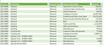
I've used Power Query to give me the table below, which is named Revenue___Expense_GRNP_Trial:
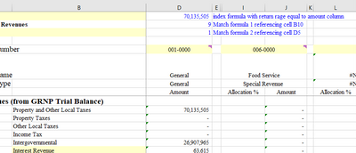
I'm using an index match match formula to pull that data into a separate tab of the same workbook with this formula
=(IFERROR(INDEX(Revenue___Expense_GRNP_Trial[[Amount]:[Amount]],MATCH('Program Revenues-Schools'!$B10,Revenue___Expense_GRNP_Trial[[Account Description]:[Account Description]],0),MATCH('Program Revenues-Schools'!D$5,Revenue___Expense_GRNP_Trial[[Fund No.]:[Fund No.]],0)),0))
That formula works for only the first "fund" in that table even though my formula is referencing that entire fund column. I say this because it won't work for any other fund in the list and if I change the sort on that original table so that the fund is descending instead of ascending, it won't even pick up fund 001-0000. Everything is formatted the same, "general" and if you look at column I, fund 006-0000 is definitely in the original data table. It's like the reference range is only looking at a limited number of rows in the table and I can't see where the error in my INDEX formula is. Any help would be appreciated!
Bridgett
- Labels:
-
Excel
-
Office 365
- Mark as New
- Bookmark
- Subscribe
- Mute
- Subscribe to RSS Feed
- Permalink
- Report Inappropriate Content
Aug 22 2022 04:00 PM
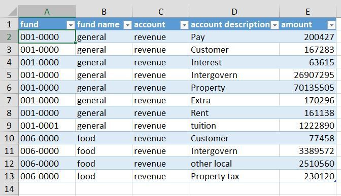
Solution=IFERROR(INDEX(Revenue___Expense_GRNP_Trial[[amount]:[amount]],MATCH(1,($B10=Revenue___Expense_GRNP_Trial[[account description]:[account description]])*(D$5=Revenue___Expense_GRNP_Trial[[fund no.]:[fund no.]]),0)),"")You can try this formula which returns the expected result in my sheet.
=IFERROR(INDEX(Revenue___Expense_GRNP_Trial[amount],MATCH(1,($B10=Revenue___Expense_GRNP_Trial[account description])*(D$5=Revenue___Expense_GRNP_Trial[fund]),0)),"")This is shorter and works as well.
I've entered the formula in cell D10 and draged across range D10:I15. Enter the formula with ctrl+shift+enter if you don't work with Office365 or 2021.
- Mark as New
- Bookmark
- Subscribe
- Mute
- Subscribe to RSS Feed
- Permalink
- Report Inappropriate Content
Aug 23 2022 06:19 AM
Accepted Solutions
- Mark as New
- Bookmark
- Subscribe
- Mute
- Subscribe to RSS Feed
- Permalink
- Report Inappropriate Content
Aug 22 2022 04:00 PM
Solution=IFERROR(INDEX(Revenue___Expense_GRNP_Trial[[amount]:[amount]],MATCH(1,($B10=Revenue___Expense_GRNP_Trial[[account description]:[account description]])*(D$5=Revenue___Expense_GRNP_Trial[[fund no.]:[fund no.]]),0)),"")You can try this formula which returns the expected result in my sheet.
=IFERROR(INDEX(Revenue___Expense_GRNP_Trial[amount],MATCH(1,($B10=Revenue___Expense_GRNP_Trial[account description])*(D$5=Revenue___Expense_GRNP_Trial[fund]),0)),"")This is shorter and works as well.
I've entered the formula in cell D10 and draged across range D10:I15. Enter the formula with ctrl+shift+enter if you don't work with Office365 or 2021.


