Index/Match Array Issue

[SisLilFeathers]

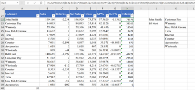
I am trying to figure out a formula for Index/Match to return the gross value for certain rows for each employee. The problem is the array for each employee can change depending on if they have or have not sold items under certain categories. (for example, some employees may not have a "internal" row  under their name on one week, but it will be there the next)

is there a way to use the employees name (ex: john smith) and have an array that will end at the next employees name (ex: Bill Hunt)

	Sales	Returns	Net Sales	Gross	GP%	Ret %
John Smith	199,166	-2,238	196,929	73,578	37.36293127	-1.136198717
Customer Pay	84,093	0	84,093	35,414	42.11262846	0
Warranty	59,366	0	59,366	24,599	41.43601366	0
Gas, Oil & Grease	13,672	0	13,672	5,095	37.26491238	0
Tires	27,009	0	27,009	4,224	15.64041825	0
Internal	5,508	0	5,508	1,933	35.08944878	0
Counter	7,091	-2,194	4,897	1,644	33.57097346	-44.80513646
Accessories	1,618	0	1,618	467	28.85099176	0
Wholesale	809	-44	766	203	26.51909892	-5.680705191
Bill Hunt	140,685	-1,299	139,386	48,271	34.63089221	-0.931945454
Customer Pay	51,502	0	51,502	20,754	40.29749634	0
Warranty	38,645	0	38,645	13,908	35.98778016	0
Wholesale	17,910	-112	17,799	4,214	23.67643936	-0.627016313
Counter	8,333	-1,033	7,300	3,079	42.17629669	-14.15570966
Internal	5,638	0	5,638	2,174	38.56080936	0
Tires	12,912	0	12,912	2,060	15.95610387	0
Gas, Oil & Grease	4,686	-52	4,634	1,732	37.3768829	-1.123915577
Accessories	1,058	-102	956	350	36.58600351	-10.66573245

[#2]

@SisLilFeathers 

You shall instruct Excel somehow which rows are with names and which are with items. As variant add helper column and mark in it each row with name; or keep blank row before each name, etc. Any formal logic you can implement, based on it to select name block.

[#3]

@SisLilFeathers wow that is a less than ideal set up for the table.  I also don't understand what you mean by "return the gross value for certain rows for each employee".  But whatever it is, may be possible if you have either a list of all employees or a list of all possible categories (and of course there is no overlap).  Here is an example I did of a cumulative sum of Gross for all subitems below that line until it reaches the next name:

=SUMPRODUCT($E22:$E$41*(ROW($E22:$E$41)>ROW($E22))*(ROW($E22:$E$41)<IFERROR(AGGREGATE(15,6,ROW($A23:$A$41)/ISNUMBER(SEARCH($A23:$A$41,CONCAT($J$22:$J$23))),1),ROW($A$41))))