Index function with Indirect function within

[JonArbuckle]

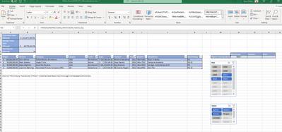
Hello, I am new to excel goin to college for it and Im struggling with a problem. I need to create a formula In cell N5, enter an INDEX function that will retrieve the name of the movie with the highest gross sales. Write the function using the INDIRECT function as the array argument and then copy the formula across to P5. Im not sure how to do this.  Any help is greatly appreciated 

[#2]

@JonArbuckle 

=INDEX(INDIRECT($F$2),MATCH(G1,movie,0))

From your screenshot i can't tell what you exactly want to do. However it's possible to combine INDEX and MATCH with INDIRECT and to drag the formula across a range.

[#3]

@JonArbuckle 

Just a guess because I can't see the sheet tabs, M5's value "Highest Grossing Movie" looks to be the name of a sheet. The #REF! might suggest you're not accounting for spaces in the sheet name and not referring to a range in that sheet.

Presuming the sheet name is "Highest Grossing Movies", this is the syntax of the INDIRECT referring to A1:A10 on that sheet. You may change the range as needed.

=INDIRECT("'"&$M$5&"'!"&"A1:A10")

The need for 2 single quotes in the INDIRECT is a good reason why it's a best practice to avoid spaces in the sheet names.

[#4]

@OliverScheurich 

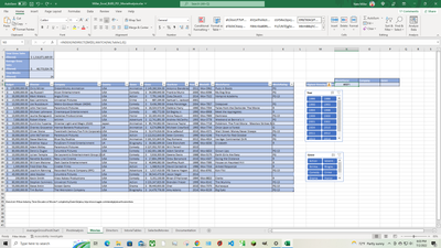
When I use that formula I get an error, did I not correctly type it in? I need to use the INDIRECT function to return a reference to a text string and my prof said I am not returning a Movie Name by referencing cell M5. The MATCH function should be looking for the maximum value in the list. Screenshot given below is the entire table with no filteres.

[#5]

@Patrick2788 

This is the entire sheet with all data unfiltered and name visible

[#6]

Are you trying to return the highest grossing movie/genre/company based on the filtered selection?

[#7]

@Patrick2788 

yes i think so. The end result should look like this:

Thank you for your help btw, much appreciated 

[#8 · Accepted solution]

@JonArbuckle 

Place in N5 and fill across:

=INDEX(Table1,MATCH(MAX(Table1[[Gross]:[Gross]]),Table1[[Gross]:[Gross]],0),MATCH(N4,Table1[#Headers],0))

[#9]

omg thank you broski if you wouldnt mind could you explain how this works, so next time I can do it on my own? Again youre a king thanks

[#10]

@JonArbuckle 

Step through the INDEX arguments:

array: Where will your return come from? We give it Table1 because your return might come from one of 3 columns depending on the MATCH results.

Row_num: MATCH(MAX(Table1[[Gross]:[Gross]]),Table1[[Gross]:[Gross]],0)

The MAX obtains the maximum value from the Gross column of the table.  Reference to the Gross column appears as Table1[[Gross]:[Gross]] so the column names do not change when you drag the fill handle right.

MATCH obtains the position of the MAX result within the Gross column. That's your row number.

Col_num: MATCH(N4,Table1[#Headers],0)

Here MATCH is obtaining the Column number where the results will come from.

Essentially, with this formula you're obtaining the Row and Column intersection of the table.