If Then Statements Across 2 Spreadsheets

[dm3333]

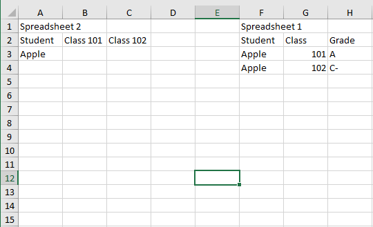
Every semester our school gives us a big report of class grades but I only need to track some students and classes. How can I set it up so I can match students names and classes and return specific grades to my spreadsheet?

So essentially:

=IF Spreadsheet1StudentName=Spreadsheet2StudentName, and Spreadsheet1Class=Spreadsheet2Class, then return Spreadsheet1Grade to Spreadsheet2Grade

Visual below (combined onto one spreadsheet for visual representation only)

[#2 · Accepted solution]

@dm3333 

With a layout like this:

In B2 on Spreadsheet 2:

=IFERROR(INDEX(Sheet1!$C$2:$C$200,MATCH(1,(Sheet1!$A$2:$A$200=$A2)*(Sheet1!$B$2:$B$200=B$1),0)),"-")

If you don't have Microsoft 365 or Office 2021, confirm the formula by pressing Ctrl+Shift+Enter.

Fill down, then to the right or vice versa.

See the sample workbook below.

[#3]

@dm3333 

I started with Power Query to avoid the use of formulas between workbooks which, rightly or wrongly, I tend to regard as somewhat fragile.

I haven't as yet used the classlist from the destination table.  It should be the basis of a filter or join, but I claim no PQ expertise!

let
    Source = Excel.Workbook(File.Contents("C:\Users\Peter\OneDrive\BigReport.xlsx"), null, true),
    Table1_Table = Source{[Item="Table1",Kind="Table"]}[Data],
    #"Changed Type" = Table.TransformColumnTypes(Table1_Table,{{"Student", type text}, {"Class", Int64.Type}, {"Grade", type text}}),
    #"Filtered Rows" = Table.SelectRows(#"Changed Type", each ([Student] <> "Banana")),
    #"Pivoted Column" = Table.Pivot(Table.TransformColumnTypes(#"Filtered Rows", {{"Class", type text}}, "en-GB"), List.Distinct(Table.TransformColumnTypes(#"Filtered Rows", {{"Class", type text}}, "en-GB")[Class]), "Class", "Grade")
in
    #"Pivoted Column"

[#4]

@dm3333 

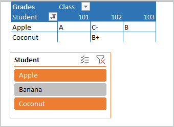
As variant you may create PivotTable with measure

Grades:=CONCATENATEX(Range, Range[Grade] )

and use slicer for filtering

[#5]

@Hans Vogelaar thank you, this worked! Very grateful. For next semester, when I run a new report for next semester's grades, is there a way to import new grade data into this, so I have a running history of grades? 

[#6]

@dm3333 

What would the data look like?

And what should the outcome look like?

[#7]

I figured out how to run a report for all time grades for specific courses, and can run that quarterly for Sheet1. For Sheet2, I'll continually update the list of students I need to track - I think this will work. The one place I'm stuck is that I only want to see grades of C, C+, B-, B, B+, A-, A, and A+ in Sheet 2. If a student didn't earn one of those grades, I want the cell to show empty for that class. The challenge is that some students fail a class and then retake, so I only want to capture in Sheet2 when they earn one of the grades above. Is there a way to do this automatically? Thanks for your reply, this is immensely helpful!

[#8]

@dm3333 

Perhaps Power Query would be better for this. Anyone?