If then not working

[MrBGL]

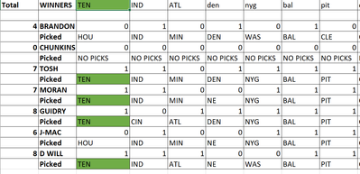
I have a spreadsheet that includes a simple If then formulae to help tally the NFL Pick Em Total. 

If the Player's team matches the "Winners" row, then the formulae should be true and a 1 should be entered in the corresponding cell. For example, D15 reads "=IF(D5=D$14,1,0)". Therefore, D15 should return as 1. That is not happening. And there are several cells that are not working properly. 

Please help!

[#2]

Hi @MrBGL 

whenever something like this happens, try to get to the root of the problem. Excel does not recognize that the two cells are the same, but you think they are the same. So, who is right? 

Check the contents of the two cells and you will find that one cell has a trailing space. "HOU" is not the same as "HOU ". So Excel is right after all. (That's a relief).

[#3]

@Ingeborg Hawighorst Wow! Such a simple solution. Not sure how I missed that. Thank you so much. 

Any ideas How I could program the sheet to give the user a predefined choice so that the data enterer cannot make that mistake?

Thanks again

[#4 · Accepted solution]

@MrBGL 

That's what data validation has been invented for. Depending on what you want to achieve, there are different data validation methods to go about this.

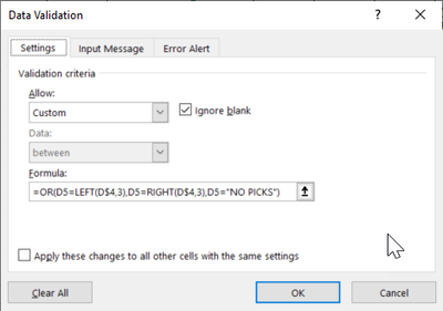
You could use a list with all the three letter codes for the teams, plus the "NO PICKS" option, or you could dynamically calculate the valid entries with a custom formula like this:

=OR(D5=LEFT(D$4,3),D5=RIGHT(D$4,3),D5="NO PICKS")

Apply that formula to the cells D5 to Q11. It will allow either the first three characters from row 5 in the current column, or the last three characters from that cell, or "No Picks".  

A list dropdown might be easier to set up and more robust, though.

 

[#5]

@Ingeborg Hawighorst THAT WAS AWESOME AGAIN!!! 

I used the drop down list.

Last question, how could can I color code the cells with the iff then statements. I.e., If 1 Green, If 0 Red or no fill?

[#6]

@Ingeborg Hawighorst 

Actually, Scratch my last question. How could I format  so that it lights up as such, i.e. If the text in the two cells match, then the result is the matched cell turns green? I know the conditional color formating will do that. But how do you scale that formula to multiple cells?

[#7]

@MrBGL You need to use a conditional formatting rule that uses a formula. Then create a formula that compares the current cell with the cell that has the value. One rule can be set up to cover all result cells, but you need to take care with the $ signs in the cell references.

An example of a rule would be

=A5=$A$1

If that rule is applied to cells A5 to A20, each row (current cell) will be compared to A1. By using the $signs, you lock in the address for A1, but the address for the current row is relative.