IF statement based on multiple columns.

[SatishBadiger]

Vendor 1	Vendor 2	Vendor 3	Vendor Master
ABC
	BCD
		CDE

Hi everyone, I'm trying to put up a IF formula for the following scenario. But I'm facing difficulty in getting the proper solution. It would be great if someone would help me to build a proper formula for this one. 
Problem statement: 
I have 3 columns for Vendors i.e Vendor 1, Vendor 2, Vendor 3. I want to put up a formula in "Vendor Master" such that IF "Vendor 1" is blank then it should return value from "Vendor 2" in "Master Vendor".
IF "Vendor 2" is also blank then it should return value from "Vendor 3".
IF "Vendor 3" is blank then it should return a string "No Vendor". 

It would also be great if someone could tell me how this can be done in Power BI as well. 

Quick response is highly appreciated.
Thanks in advance.  

[#2]

@SatishBadiger 

I'm pretty sure someone will have a more eloquent formula but this can be done with nested IF formula - see attached example

=IF($A2>"",$A2,IF($B2>"",$B2,IF($C2>"",$C2,0)))

[#3]

@SatishBadiger 

If under Power BI you mean transformation in Power Query, you may add custom column as

= Table.AddColumn( Source,
   "Vendor Master",
   each List.RemoveNulls(Record.FieldValues( _ )){0}  )

[#4]

Hey @Charla74, thank you so much this worked!!

[#5]

Hi @SatishBadiger 

For PowerBI/Power Query, similar to @Sergei Baklan with the "No vendor" exception:

= Table.AddColumn(PreviousStep, "Vendor Master", each
    try List.RemoveNulls(Record.ToList(_)){0} otherwise "No vendor"
)

[#6]

@Sergei Baklan 

I have 15 other columns in my dataset. Will this code still work?

[#7]

@SatishBadiger 

Record.FieldValues and Record.ToList take a Record ("row" if you prefer) and return a List containing all  values from that Record, whatever the number of columns is

[#8]

@SatishBadiger
If you have Filter and each row has only one entry, you could use
=FILTER(A2:C2,A2:C2<>"")

[#9]

Hi @Charla74 ,

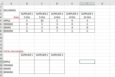
How about if statement to add multiple columns? how to summarize it.

Thank you so much.

[#10]

@RaquelJ 

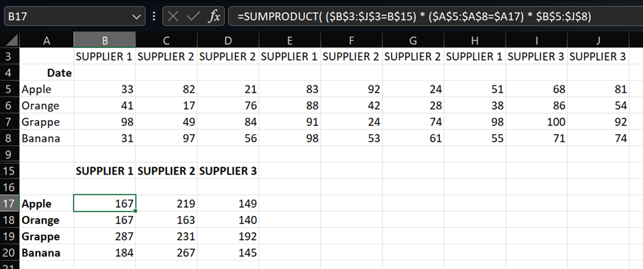
in B17 then copy right and dow:

=SUMPRODUCT( ($B$3:$J$3=B$15) * ($A$5:$A$8=$A17) * $B$5:$J$8)

[#11]

@RaquelJ 

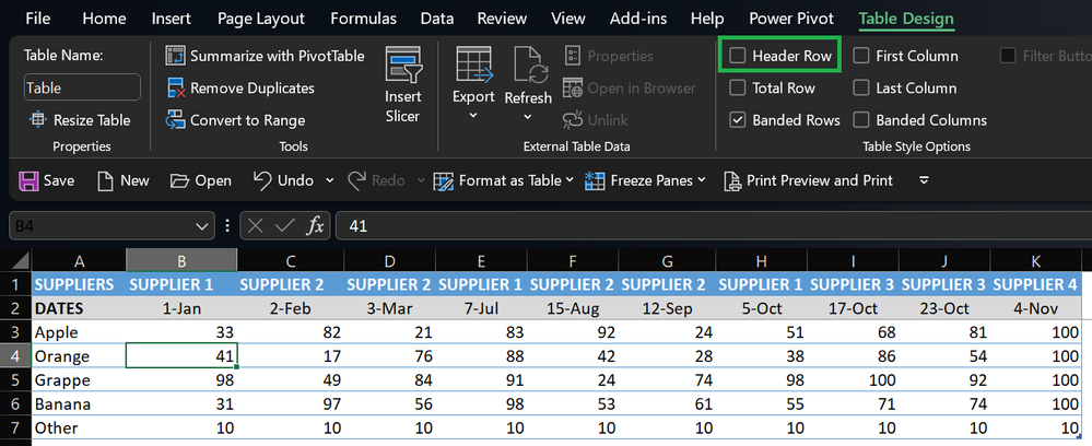
If you're on Windows with Excel >/= 2016 or on Mac with Excel 365 (up to date) there's a better solution (sample attached) without changing the way you record data. The below data are formatted as a Table where the Header isn't displayed:

That Table is unpivoted with Get & Transform (aka Power Query). The resulting table is used as the Source of a Pivot Table:

Main benefits: As you add new columns/rows to the data Table it's dynamically resized, picking your additional Suppliers and/or Products, no more formula, Products and Suppliers are automatically sorted in the pivot table...

[#12]

Your given is lacking context, i.e. why are the vendors in different rows what is the reason or basis for that, maybe that reason/basis would also become an integral part of the formula solution?

[#13]

@SatishBadiger 

So the geographical context is "Vendor Master"

Logic context is if the vendor # 2 is blank, the system or vendor admin does not promote a vendor 3 to vendor 2 if vendor 2 is blank for some valid reason?

What is the logic behind having alternate vendors? Pricing? Stock availability? Other?

Does the company policy allow the system to have a vendor 3 when vendor 2 is blank?

Why would vendor 1 be blank? when there is vendor 2 and vendor 3?

The only reason each vendor is in a different row is because it is a different company and not the same company in a different location/store

"I have 3 columns for Vendors i.e Vendor 1, Vendor 2, Vendor 3. I want to put up a formula in "Vendor Master" such that IF "Vendor 1" is blank then it should return value from "Vendor 2" in "Master Vendor"."  - Gives me the impression that the vendor is the same company in a different location.

What is the basis on the condition that there is "no vendor"?