IF/OR INDEX MATCH STATEMENT

[kdwork]

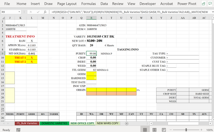
Please, Please Help.  I have my last major hurdle to fix on a complicated project I have been trying to get done for way too long between busy times.  I am using Windows 10 Enterprise with Excel 365

In the attached file on the Tab New Office Copy cell R9 I have the following formula that I need to look at two different tabs (ITL_Bulk Varieties and Domestic Varieties) depending on what Brand is selected in Cell E3.  If E3 selects CAN.INTL or BULK, it needs to search tab ITL_Bulk Varieties.  All the other brand selections would search tab Domestic Varieties.  My formula works perfectly for the brands searching the Domestic Varieties (green portion of the formula).  However when I choose CAN.INTL or BULK, the formula is not performing the portion highlighted in Red.

=IF(OR($E$3={"CAN.INTL","BULK"}),IFERROR(OFFSET('ITL_Bulk Varieties'!$A$1,MATCH(1,INDEX(($E$3='ITL_Bulk Varieties'!$A$2:$A$654)*($C$6='ITL_Bulk Varieties'!$E$2:$E$654),,),0),MATCH($S$9,'ITL_Bulk Varieties'!$A$1:$CC$1,0)-1,1,1),100-R10-R11-R12),IFERROR(OFFSET('DOMESTIC VARIETIES'!$A$1,MATCH(1,INDEX(($E$3='DOMESTIC VARIETIES'!$A$2:$A$600)*($C$6='DOMESTIC VARIETIES'!$E$2:$E$600),,),0),MATCH($S$9,'DOMESTIC VARIETIES'!$A$1:$CP$1,0)-1,1,1),100-R10-R11-R12))

The formula is dependent on what variety is selected in C6.  The file is saved with the Brand CAN.INTL selected for E3 and Variety INTL MISC ND AN 25KG selected for C6.  Cell R9 needs to perform the formula in red above since it is not finding any info in the blue portion of the formula.  If you go to C6 and select the Variety above the one that is saved (INT MISC DORM AN 25KG), the formula is performing the portion in blue correctly.

What am I missing?  I know it is a complicated formula and it would be much easier if all my data was on one spreadsheet, but because of the needs of the business, I need to have it separated.

Please help.  I am desperate to put this project to bed and have it out of my hair!

[#2]

@kdwork 

In your formula

=IF(
  OR( $E$3={"CAN.INTL","BULK"} ),
 IFERROR( OFFSET( 'ITL_Bulk Varieties'!$A$1,
                  MATCH( 1, INDEX( ($E$3='ITL_Bulk Varieties'!$A$2:$A$652 )*
                                   ($C$6='ITL_Bulk Varieties'!$E$2:$E$652),,),
                         0 ),
                  MATCH( $S$9,  'ITL_Bulk Varieties'!$A$1:$CC$1,0) -1,
                   1,1),
 100 - R10 - R11 - R12),
 IFERROR( OFFSET( 'DOMESTIC VARIETIES'!$A$1,
                  MATCH( 1, INDEX( ($E$3='DOMESTIC VARIETIES'!$A$2:$A$600)*
                                   ($C$6='DOMESTIC VARIETIES'!$E$2:$E$600),,),
                          0 ),
                  MATCH( $S$9, 'DOMESTIC VARIETIES'!$A$1:$CP$1, 0) - 1,
                  1,1),
 100 - R10 - R11 - R12)
)

MATCH() in first portion finds something, thus OFFSET() returns value, thus "red" portion is not triggered by IFERROR()

[#3]

@kdwork  so you say it doesn't work but it is working exactly as you designed it in that it finds the corresponding row and col and offsets to the corresponding cell.  That cell happens to be blank which it takes as 0.  That is not an error and hence doesn't use that RED portion of the formula.  If you really want that to happen a simple trick is to add 1/1/ in front of it to force a divide by 0 error:

=IF(OR($E$3={"CAN.INTL","BULK"}),IFERROR(1/(1/Value(OFFSET('ITL_Bulk Varieties'!$A$1,MATCH(1,INDEX(($E$3='ITL_Bulk Varieties'!$A$2:$A$654)*($C$6='ITL_Bulk Varieties'!$E$2:$E$654),,),0),MATCH($S$9,'ITL_Bulk Varieties'!$A$1:$CC$1,0)-1,1,1))),100-R10-R11-R12),IFERROR(OFFSET('DOMESTIC VARIETIES'!$A$1,MATCH(1,INDEX(($E$3='DOMESTIC VARIETIES'!$A$2:$A$600)*($C$6='DOMESTIC VARIETIES'!$E$2:$E$600),,),0),MATCH($S$9,'DOMESTIC VARIETIES'!$A$1:$CP$1,0)-1,1,1),100-R10-R11-R12))

that said I suspect you might need the same for the second half of the formula even though you say it is working.

That all said, you could also make the whole thing cleaner/more simple using the new LET statement 

=LET(tab,IF(OR($E$3={"CAN.INTL","BULK"}),'ITL_Bulk Varieties'!$A$1:$CC$652,'DOMESTIC VARIETIES'!$A$1:$CP$600),
        brandCol, INDEX(tab,,1),
        varietyCol, INDEX(tab,,5),
        headerRow, INDEX(tab,1,),
        irow, MATCH(1,($E$3=brandCol)*($C$6=varietyCol),0),
        icol, MATCH($S$9,headerRow,0),
        foundCell, INDEX(tab,irow,icol),
        altResult, 100-R10-R11-R12,
        IFERROR(IF(foundCell=0,altResult,foundCell),altResult)
        )

I put that version in col F just to the right of the original

[#4 · Accepted solution]

@kdwork 

=IFERROR(
  INDEX('ITL_Bulk Varieties'!$AK$2:$AK$8,
    MATCH($C$6,'ITL_Bulk Varieties'!$E$2:$E$8,0)),"")
&IFERROR(
  INDEX('DOMESTIC VARIETIES'!$AK$2:$AK$32,
    MATCH($C$6,'DOMESTIC VARIETIES'!$E$2:$E$8,0)),"")

[#5]

Your 1/1/Value worked beautifully. With the Let statement, if the columns on the Varieties tab were to be moved/rearranged, then this statement would have to be updated, correct?

[#6]

yes if the Brand and Variety columns moved they would need to be updated but you could instead used MATCH() to find the corresponding column index based on the header name.

[#7]

@kdwork 

try this:

=IF(OR($E$3={"CAN.INTL","BULK"}),IF(OR(FILTER(INDEX(('ITL_Bulk Varieties'!$AI$2:$AI$8,'ITL_Bulk Varieties'!AJ2:AJ8),,,MATCH('NEW OFFICE COPY'!$S$9,'ITL_Bulk Varieties'!$AI$1:$AJ$1,0)),('ITL_Bulk Varieties'!$A$2:$A$8='NEW OFFICE COPY'!E3)*('ITL_Bulk Varieties'!$E$2:$E$8='NEW OFFICE COPY'!C6))=0,ISERROR(FILTER(INDEX(('ITL_Bulk Varieties'!$AI$2:$AI$8,'ITL_Bulk Varieties'!AJ2:AJ8),,,MATCH('NEW OFFICE COPY'!$S$9,'ITL_Bulk Varieties'!$AI$1:$AJ$1,0)),('ITL_Bulk Varieties'!$A$2:$A$8='NEW OFFICE COPY'!E3)*('ITL_Bulk Varieties'!$E$2:$E$8='NEW OFFICE COPY'!C6)))),100-R10-R11-R12,FILTER(INDEX(('ITL_Bulk Varieties'!$AI$2:$AI$8,'ITL_Bulk Varieties'!AJ2:AJ8),,,MATCH('NEW OFFICE COPY'!$S$9,'ITL_Bulk Varieties'!$AI$1:$AJ$1,0)),('ITL_Bulk Varieties'!$A$2:$A$8='NEW OFFICE COPY'!E3)*('ITL_Bulk Varieties'!$E$2:$E$8='NEW OFFICE COPY'!C6))),IFERROR(OFFSET('DOMESTIC VARIETIES'!$A$1,MATCH(1,INDEX(($E$3='DOMESTIC VARIETIES'!$A$2:$A$600)*($C$6='DOMESTIC VARIETIES'!$E$2:$E$600),,),0),MATCH($S$9,'DOMESTIC VARIETIES'!$A$1:$CP$1,0)-1,1,1),100-R10-R11-R12))

You can also change the $S$9 to Minima G

cheers