Icon sets based on columns with dates giving me grief

[Trish_Hopkins]

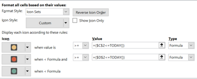
I have played around and can get one of the 3 "stop lights" to work, but not all.

The intent is to have a visual when a task hasn't been started (no dates in either column C or D); Have started (date in Verified by #1), but not in Verified by #2); task complete (dates in both Verified #1 and verified by #2)

STATUS	BT	VERIFIED BY #1	VERIFIED BY #2
YELLOW	1	11/04/2023
GREEN	2A	11/04/2023	12/04/2023
RED	2B

I know the following doesn't work. Any advice?

[#2 · Accepted solution]

@Trish_Hopkins 

So far, I understand you are trying to use icon sets in a spreadsheet to visually represent the status of tasks based on dates in columns C and D.

If this is correct...

You can use conditional formatting with a formula to achieve your desired result.

Here’s how you can do it:

1. Select the cells in the Status column that you want to apply the formatting to.
2. On the Home tab, click Conditional Formatting > New Rule.
3. In the New Formatting Rule dialog box, select “Use a formula to determine which cells to format”.
4. In the formula field, enter a formula that returns TRUE or FALSE based on the values in columns C and D. For example, to display a yellow icon when there is a date in column C but not in column D, you could use the formula =AND(ISNUMBER(C1),NOT(ISNUMBER(D1))).
5. Click Format and select the yellow icon from the Icon Sets.
6. Repeat steps 2-5 for the other two icon sets (red and green), using appropriate formulas for each.

If it's not what was wanted, please include the following info to help others answer your question:

Welcome to your Excel discussion space!

I hope this helps!

[#3]

@NikolinoDE Perfect! This does the conditional formatting and will work for now. I was hoping for te traffic light Icon Set, but this will work.

[#4]

I am glad that I could help you.
I wish you continued success with Excel!