How to use conditional formatting to highlight information after using =DATEDIF to calculate age?

[Jeffkcl]

Hi everyone, this is my first time here.

I already using =DATEDIF(E3,TODAY(),"Y") & "Y" & DATEDIF(E3,TODAY(),"YM") & "M" to calculate their age, after that, I would like to use conditional formatting to highlight those results over 59Y05M, what should I do?

Thanks!

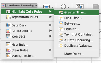
[#2 · Accepted solution]

@Jeffkcl You can use rule from the "Highlight Cells" group, Greater Than...

And then just type 59Y05M in the box to the right of "greater than". It will create rule like this:

 

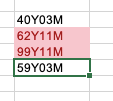
and result in formatting like this:

The above screenshots were taken on a Mac, but it's very similar on the PC version of Excel.

[#3]

Oh! It's work! But it didn't work before,
Anyway, thanks so much!