How to make a cell dependant on another, and perform different calcs based on the orginal cell?

[CobyCurtis]

Hi,

My excel skills are average at best and I am trying to track my trades better so I have tried to create a sort of ledger; however I have hit a brick wall.
I am trying to make the spreadsheet that is as simple as possible and have it be as autonomous as possible.
My question is the following; is it possible to have the multiple cells within the same row, dependent on one single cell, and if so, how? The best way for me to explain is to use an example:

If cell A1 says 'LSE' then the following formulas will apply in the following cells within the row:
Cell P1 =(L1*T1)*M1
Cell Q1 =P1
Cell W1 =((T1-U1)*L1)
Cell X1 =W1/Summary!F5
and so on..

If cell A1 says 'NYSE' then the following formulas will apply in the following cells within the row:
Cell P1 =(L1*T1)*M1
Cell Q1 =P1*0.81
Cell W1 =((T1-U1)*L1)*0.81
Cell X1 =W1/Summary!F5
and so on..

If cell A1 says 'EPA' then the following formulas will apply in the following cells within the row:
Cell P1 =(L1*T1)*M1
Cell Q1 =P1*0.88
Cell W1 =((T1-U1)*L1)*0.88
Cell X1 =W1/Summary!F5
and so on..

On my spreadsheet there are a total of 12 cells within the row that I want linked to the initial cell (LSE,NYSE or EPA) and automatically update.

Also, I am trying to make it so it works on any row, so that if I click on Cell A4, and select NYSE, the cells within row 4 display the formulas:
Cell P4 =(L4*T4)*M4
Cell Q4 =P4*0.81
Cell W4 =((T4-U4)*L4)*0.81
Cell X4 =W4/Summary!F5
and so on..

Or if I click cell A9 and select EPA, the cells within row 9 and display the following formulas:
Cell P9 =(L9*T9)*M9
Cell Q9 =P9*0.88
Cell W9 =((T9-U9)*L9)*0.81
Cell X9 =W9/Summary!F5
and so on..

I have tried the following formula:

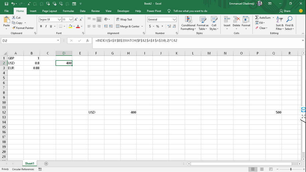
=IF(F12="GBP",Q12)=IF(F12="USD",Q12*0.8)=IF(F12="EUR",Q12*0.88)

However, all that I get back is 'TRUE'. I want the calculation not a confirmation that the formula is correct :\

I hope I have explained this well, and of course, thank you in advance for any help it is much appreciated.

Cheers,

C

[#2]

Hi @CobyCurtis 

You can adjust the formula to 

=IFS(F12="GBP",Q12,F12="USD",Q12*0.8,F12="EUR",Q12*0.88)

With this, you will get the intended value.

However, I believe you can set up your data in a better way, so you won't hardcode the numbers in your formula, for example, have a table for the values of each GBP, USD and EUR.

You can then use INDEX and MATCH or VLOOK (XLOOK is also useful)

=INDEX($A$1:$B$3,MATCH($F$12,$A$1:$A$3,0),2)*$Q$12

Cheers,