How to have column values arranged in pivot as in the picture?

[jthomsoun]

Hello,

In pivot, I basically want to arrange 2 values - Agent & Ticket ID.

The current view is like this,

I want to view as like this,

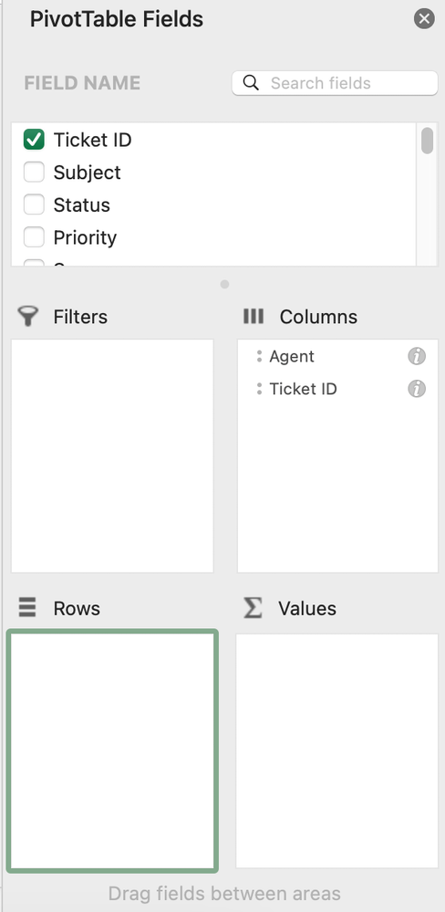
The pivot is currently like this,

What should I do to get the expected view?

Someone, please help.

Regards,

Thomson

[#2]

Hi@jthomsoun 

No way with a PivotTable and the 2 fields you exposed + bad luck you're on Mac (a cheaty option exists on Windows with Power Query). Alternative if you run 365:

in E4:

=TicketsByAgent(TableSource[Agent], TableSource[Ticket ID])

in K4:

=TicketsByAgent(TableSource[Agent],TableSource[Ticket ID],TRUE)

Where TicketsByAgent is LAMBDA function:

=LAMBDA(Agents, Tickets, [remove_duplicates],
  LET(
    StackAgentTickets, LAMBDA(seed, agent_k,
      LET(
        tickets_agent_k, FILTER(Tickets, Agents=agent_k),
        HSTACK(seed, SORT(IF(remove_duplicates, UNIQUE(tickets_agent_k), tickets_agent_k)))
      )
    ),
    u_Agents, TOROW(SORT(UNIQUE(Agents))),
    VSTACK(u_Agents, IFNA(DROP(REDUCE("",u_Agents, StackAgentTickets),,1),""))
  )
)

[#3]

@jthomsoun 

As non Mac user I missed the recent General Availability of the Power Query Editor for Excel Mac

The cheaty option:
- Load the Source Table to Power Query
- Group the table by Agent
- Sort each group Ticket IDs
- Add an Index to each Group
- Expand all fields
- Close & Load To... > PivotTable Report

In the PivotTable:
- Agent Index to Rows
- Agent to Columns
- Ticket ID to Values

Then Hide the column that holds the Agent Index:

In the attached file 2 Power Queries that keep or remove duplicates
All query steps done with the User Interface (shorter version exists with the Advanced Editor)