How to get row data if matching specific column criteria

[FaisalExcell]

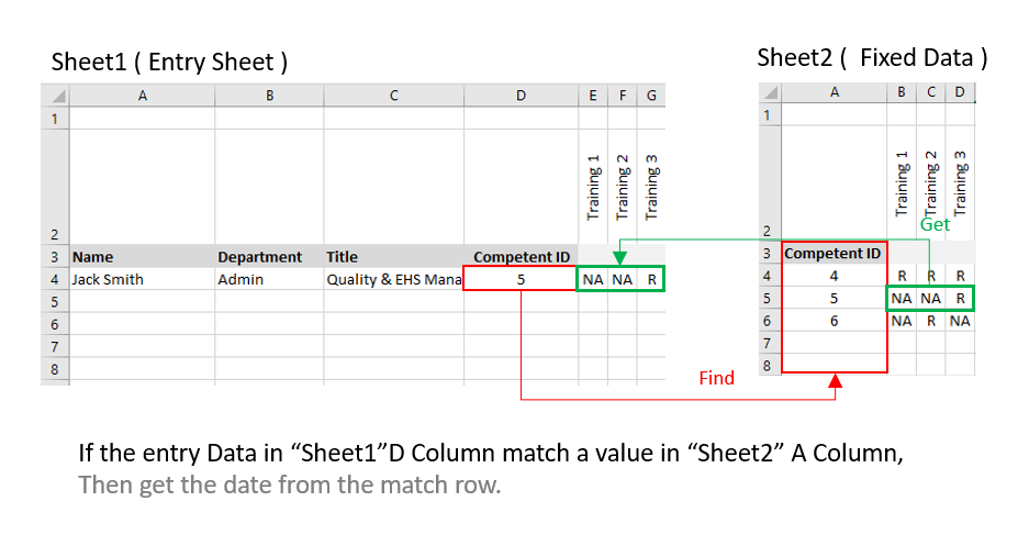
Im really struggling on writing the correct formula here appreciate if i could get a help

[#2 · Accepted solution]

@FaisalExcell See a mock-up of your schedule attached, offering three different approaches. VLOOKUP, XLOOKUP and INDEX/MATCH.

[#3]

You are the Best!!!! thank you my dear for your quick respond

[#4]

Hi @Riny_van_Eekelen 

I have used the VLOOKUP, but now i found a problem when i drag to fill to the next cell horizontally.

if the VLOOKUP is first entered in cell F5 as below

=VLOOKUP($D5,'Competency Requirement'!$C$5:$KS$100,2,FALSE)

Then i would like it to become as below if I drag it horizontally to G5

=VLOOKUP($D5,'Competency Requirement'!$C$5:$KS$100,3,FALSE)

the same for the next till end of the training list.

i have attached the file for better look.

[#5]

@FaisalExcell Best to add a MATCH function to make the column definition dynamic:

=VLOOKUP($D5,'Competency Requirement'!$C$5:$KS$100,MATCH(F$3,'Competency Requirement'!$C$3:$KS$3,0),FALSE)

To make it all easier to read and maintain, however, consider creating named ranges for the lookup range (e.g. CompReq) and the column headers (e.g. TRheader). Then, the formula could look a lot more user-friendly, like:

=VLOOKUP($D5,CompReq,MATCH(F$3,TRheader,0),FALSE)

Did just that in your original file. See attached.

[#6]

Perfect ! Thank you again for your help

[#7]

@FaisalExcell You're welcome!

[#8]

Hey @Riny_van_Eekelen i promise this will be my last :D

in the Employee Profile tab I'm trying to get the confirmation date from Employee Training Matrix, i managed by luck to get the requirement need but when i applied the same used formula to the date i get #VALUE 

[#9]

@FaisalExcell In the last part of the formula ('Employee Training Matrix'!F6:KS164)), you should change the first cell in the return_array to F5 so that the size matched the size of the lookup_array.

[#10]

Hi @Riny_van_Eekelen  but that will get me the information of the requirement F5, i want to get the dates from F6.

[#11]

@FaisalExcell Aha, I see. Try this one in stead:

=TRANSPOSE(XLOOKUP(C4,'Employee Training Matrix'!A5:A164,'Employee Training Matrix'!F6:KS165))

 The Lookup_array is in row 5:164 and return array in row 6:165. Still the same array size, but shifted one row between them.

[#12]

@Riny_van_Eekelen Thanx Riny i have figured that out during the weekend.

=TRANSPOSE(XLOOKUP(C4,'Employee Training Matrix'!A5:A164,'Employee Training Matrix'!F6:KS165))

but the empty cells are showing 0 when transposing, how can i add IF in middle of the formula to Show "--" if empty cells ?

[#13]

@FaisalExcell Try this:

=IF(C9#="NA","--",TRANSPOSE(XLOOKUP(C4,'Employee Training Matrix'!A5:A164,'Employee Training Matrix'!F6:KS165)))