How to Create LOV with category with corresponding sub-category

[Julius575]

Hi Excel Community,

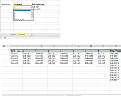
Hope you can help me with my concern, i have here my list of values for category and sub-category for figure 1, all i want is to reflect in figure 2, when i input in the category column,  the LOV for sub-category should be reflected accordingly to respected category.

For Example:

when i input  Berth Maneuvering (column R) for category (LOV), LOVs for subcategory should reflect in the subcategory (column S)

figure 1

figure 2

[#2 · Accepted solution]

@Julius575 Added a workbook with two examples of Data Validation. The first one uses a structured table with all the options and dynamic array functions UNIQUE and FILTER. The second example uses a more traditional method with named ranges, though it's less flexible and requires more maintenance. 

[#3]

thank you Riny Van! it works

[#4]

@Riny_van_Eekelen 

i tried to use the alternative, i added categories but it couldn't reflect the subcategory that i added, hope you can help me with this.

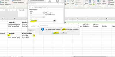
i used function INDIRECT in the data validation for sub-category.

[#5]

@Julius575 But did you create named ranges for x,y,z, etc? And better to change the sub-categories in the example. Then you can at least see what you are looking at when you click in the drop-down in the cell next to "y". For example, use sub-categories y1 to y5, and z1 to z5.

[#6]

@Riny_van_Eekelen 

i already did to change sub-categories,

when i do the data validation, there's an error occurred pls see below screenshot

[#7]

Hi Riny,

Attached file, already plot data for sub-cat in the "option" sheet.

kindly check "selection" sheet on the sub-category with the red-highlight it doesn't shows LOV for sub-cat.

[#8]

@Julius575 Fixed. Although you created the various option lists, you did not create Named Ranges for them. I did that in the attached file. The easiest way to do it yourself is the select a list with options including the header, and then on the Formula Ribbon in the Define Names group click on "Create from selection" and confirm that the name of range is in the top row.

Repeat this for every list. You could select the entire range with options (incl. the headers) and do it all at once, but than you include blanks at the end of all lists that are shorter than the longest one. You can click on the Name Manager symbol to view all named ranges in the current workbook.

[#9]

Hi Sir,

lastly

The category for on-time doesn't work, other category are okay now.

[#10]

@Julius575 Sorry! missed than one. Named ranges may not start with a number, contain spaces or any special characters. Such starting numbers will be preceded by an underscore. Spaces and special characters will be replaced by an underscore. So, change the header "On-time" to "On_time". Then it shall work.

[#11]

Hi Sir,

It works!
Thank you so much for your help.
Appreciate it!