- Home
- Microsoft 365
- Excel
- Re: How to categorize companies in Excel
How to categorize companies in Excel
- Subscribe to RSS Feed
- Mark Discussion as New
- Mark Discussion as Read
- Pin this Discussion for Current User
- Bookmark
- Subscribe
- Printer Friendly Page
- Mark as New
- Bookmark
- Subscribe
- Mute
- Subscribe to RSS Feed
- Permalink
- Report Inappropriate Content
Nov 18 2021 01:53 AM
Dear All,
First off; thank you for taking the time to help me.
I've been looking for the right fix for my problem but can't wrap my head around it.
Solution: formula which categorizes companies, in category A, B or both, based on money spent.
Situation:
I've got three excel files. Excel file 1 contains companies of which i want to know whether they belong to Category A, Category B or both. The only way for me to know whether the company named in excel 1 belongs to one of the categories is to look up the name or number in Excel 2 & 3 and check whether money was spent on them. If excel 2 states a positive amount then the company belongs to category A, if excel 3 states a positive amount then the company belongs to category B. However, if excel 2 & 3 state a positive amount then the company belongs to category A & B.
(please read excel files containing data)
Already tried:
- I've used the IF function and Vlookup function
Vlookup
1. Look up the company name of excel 1 in excel 2
2. If found name the amount spent
IF function
1. If the amount is >=0.01
2. If true then return "category A"
3. If False then return "no spend or Negative"
I have done the same for category B but repalced excel 2 for excel 3.
Problems encountered:
I have encountered the following problems
- Because of wrongly spelled names or case sensitivity some suppliers are not found and excel returns #N/A
- Excel 2 and 3 might contains multiple dates on which money has been spent. With Vlookup the first money spent is found and returned. So if the first money spent is -20, excel will return "No Spend or Negative". However, the other dates have spent which are positive (e.g. +40 or +50). Because Vlookup directly takes the first found value and doesn't look further, a company can be categorised incorrectly.
- If the company is not found in excel 2 or 3, the function returns #N/A.
- some companies have nagetive money spent but in total it is positive. For example; first time money spent on a company is -20, the second time it is 40 and the third time it is 10. The total is still positive because -20 + 40 +10 = 30 spent.
Actions taken:
I have tried the following solutions.
- To prevent wrongly spelled names, I have replaced the name with supplier number. Shortly said; supplier number will be looked up in excel 2 and 3 instead of name. However, i still receive the same output.
Excel Files and the containing data
Excel 1 contains
- Approved companies
- Company name
- Company number
- Bunch of other irrelevant data
Excel 2 contains
- Money spent on companies which belong to category A
- Company name
- Company number
- Amount of money spent
- Currency
- bunch of other irrelevant data
Excel 3 contains
- Money spent on companies which belong to category B
- Company name
- Company number
- Amount of money spent
- Currency
- bunch of other irrelevant data
Again thank you for helping me.
- Labels:
-
Excel
-
Formulas and Functions
-
Training
- Mark as New
- Bookmark
- Subscribe
- Mute
- Subscribe to RSS Feed
- Permalink
- Report Inappropriate Content
Nov 18 2021 03:28 AM
That's more job for Power Query. If with formulas when use SUMIFS(), not lookup functions.
- Mark as New
- Bookmark
- Subscribe
- Mute
- Subscribe to RSS Feed
- Permalink
- Report Inappropriate Content
Nov 18 2021 03:35 AM
- Mark as New
- Bookmark
- Subscribe
- Mute
- Subscribe to RSS Feed
- Permalink
- Report Inappropriate Content
Nov 18 2021 04:14 AM
Power Query is part of Excel, this functionality is under Get & Transform tab.
Again, you may use SUMIFS() formulas to return companies spending.
- Mark as New
- Bookmark
- Subscribe
- Mute
- Subscribe to RSS Feed
- Permalink
- Report Inappropriate Content
Nov 19 2021 11:47 AM
Power Query as well as Visual Basic macro language are both parts of an Excel installation but they demand knowledge very different from the spreadsheet.
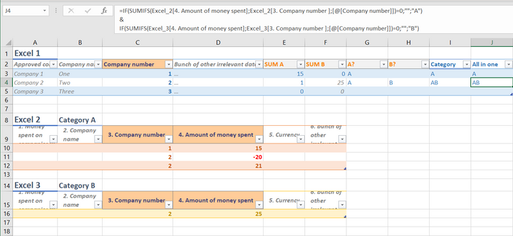
Using SUMIFS to find the total amount spent for each company mentioned in table Excel_1 will calculate the sum no matter their order respective tables.
If the amount is greater than zero, the IF statement should result in a letter, A or B.
The two are then concatenated using &.
=IF(SUMIFS(Excel_2[4. Amount of money spent];Excel_2[3. Company number ];[@[Company number]])=0;"";"A")
&
IF(SUMIFS(Excel_3[4. Amount of money spent];Excel_3[3. Company number ];[@[Company number]])=0;"";"B")
Excel_1 columns E to I calculates this step by step while col J makes it all in one formula.
If you are not using 'pyamas' tables, change the column references to your columns, eg cell J3 using ranges in other files like
=IF(SUMIFS([Book2]Sheet1!$D:$D;[Book2]Sheet1!$C:$C;C3)=0;"";"A")
&
IF(SUMIFS([Book3]Sheet1!$D:$D;[Book3]Sheet1!$C:$C;C3)=0;"";"B")
- Mark as New
- Bookmark
- Subscribe
- Mute
- Subscribe to RSS Feed
- Permalink
- Report Inappropriate Content
- Mark as New
- Bookmark
- Subscribe
- Mute
- Subscribe to RSS Feed
- Permalink
- Report Inappropriate Content
Nov 23 2021 12:00 AM
