How to apply conditional formatting for multiple relative cells

[DSK Chakravarthy]

Hi Experts,

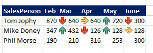
I'm planning to prepare a sheet with the below data and it is taking around 15+ clicks for each cell to show the arrow mark.

The logic for the arrow mark is the comparison with the previous month's value. But, it is not accepting the relative reference while constructing the rule.

When changed the $E$8 to E8, I get the following error

16+ clicks for each cell is a mundane activity and I have 100s of rows to compare and generate a dashboard.

Thanks for reading. Appreciate any thoughts. I have read previous posts in this directions, but, none are in similar lines that my situation.

Regards,

[#2]

@DSK Chakravarthy 

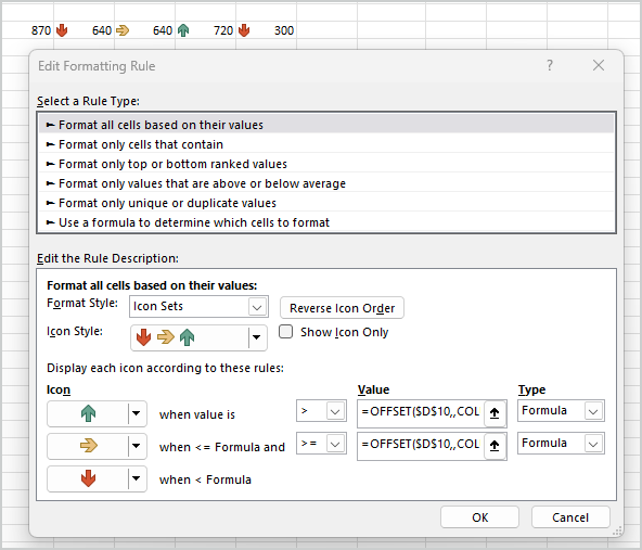
We can't use relative references for such conditional format, but we may use OFFSET(). The idea is here Conditional Formatting Icons with Relative References – Daily Dose of Excel

For your sample

[#3]

Thank you for the quick inputs. Yes, that is working for one row. But, on one condition, that there should not be data, due to copying the cell. So, initially, I have to format the cells and feed the data into the cells.

Now the challenge is for multiple employees. I have about 100s of rows. When I copy the previous row, the offset reference is still remaining with previous cell. Thus, I have to format the initial cell of the row again and then copy that to the next cell.

Is there any other way to

point 1) avoid multiple single copy cell mechanism?
point 2) use it with multiple rows

[#4]

@DSK Chakravarthy 

We may modify rule formula as

=OFFSET($D$10, ROW()-ROW($D$10),COLUMN()-COLUMN($D$10)-1)

and be sure rule is applied only to the cell E10

Using format painter apply the rule to other cells in this row and next row. Let assume first row won't be copy/pasted.

Now if we copy paste one of next rows, e.g. D14:H14 to D11:H11 and check the rule in any cell of these rows we see that rangy to apply is expanded

which give incorrect behaviour. We need to apply icons rule to one cell only. For that select first row (E10:H10), double click on format painter icon and apply rules to rows which you copied and into which you pasted, in our case is just click with format painter on E14 and E15.

Check again, rue is applied to one cell only and works correctly

Range to apply is usually expanded if you copy/paste last row with data to the next empty one. If copy/paste row from the middle of data it shall work without correction. Didn't play with all scenarios (deleting, inserting, etc). If in your scenario it doesn't work you always may apply format from unchanged first row.