How do I use 2 sets of Data (one as a criteria) without nesting a bunch of =X into the formula?

[nick1989]

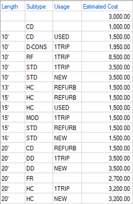
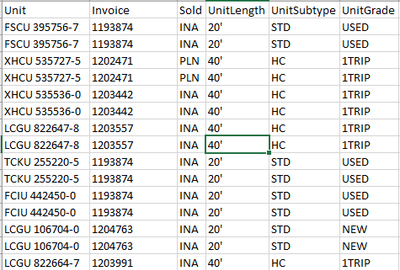
I have a data set that I need to look up the estimated cost based on 3 criteria which is roughly 80 lines of Data in a table format where the cost is based on length, subtype, and condition without manually entering all of the different values in the formula?

Example of the Criteria:

Example of the Data set I want to look up all 3 criteria in and have the estimated cost returned from:

[#2]

@nick1989 

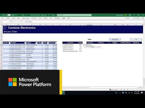
This sounds very much like a job for the relatively new FILTER function. Here's a good YouTube intro to that function (it's where I learned how to use it): https://www.youtube.com/watch?v=9I9DtFOVPIg

If you prefer reading to viewing, here's another good resource: https://exceljet.net/excel-functions/excel-filter-function

The FILTER function will enable you to search through a table with multiple criteria.

[#3]

@nick1989 

Depends on your Excel version/platform, in general that could be like

=INDEX( EstimatedCost,
   MATCH(1, INDEX(
         (UnitLength=LengthRange)*
         (UnitSubtype=SubtypeRange)*
         (UnitGrade=UsageRange), 0), 0)
)

If you could provide sample file without sensitive information it'll be easier to explain details.