How can I match two columns in a table to pull from a corresponding 3rd column?

[Houston-Jack]

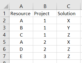
I have a table of rows sorted by "project" where a Project can have multiple solution components represented in separate rows, each with a resource assigned.  As in:

For example: I need to find the resource value ("D") in a row where project value = 2 and Solution =Z

A LookUp on Project or Solution will not isolate the other variable.  It might take nesting of the LookUps that I haven't figured out yet.

Thanks

[#2]

@Houston-Jack 

Two way lookup in Excel. 

[#3 · Accepted solution]

@Houston-Jack Replicated your table and used the new FILTER function to find the Resource based on the combination of Project and Solution. If your Excel version does not recognise it, a more traditional approach need to be taken.

[#4]

Thanks for the reply, @Detlef Lewin , but my need was to match on values in two columns of the same row to obtain the value in a third column of that row.  @Riny_van_Eekelen  provided an elegant solution to that in the post below.

[#5]

Thanks for the elegant solution, @Riny_van_Eekelen, I was a bit hung up on the AND of the two logical expressions.  Your solution also provided a means of finding all the related matches and not stopping on just the first result.  I was able to use TEXTJOIN to assemble the results in a single cell.  My final formula looked like this:

=TEXTJOIN(" ",TRUE,FILTER('Estimate Data'!$D:$D,('Estimate Data'!$I:$I=$B3)*('Estimate Data'!$K:$K=Sheet1!C$2),""))

[#6]

@Houston-Jack Very good! Glad I could help.