- Home
- Microsoft 365
- Excel
- How can I get my cell to automatically change based on referenced date data?
How can I get my cell to automatically change based on referenced date data?
- Subscribe to RSS Feed
- Mark Discussion as New
- Mark Discussion as Read
- Pin this Discussion for Current User
- Bookmark
- Subscribe
- Printer Friendly Page
- Mark as New
- Bookmark
- Subscribe
- Mute
- Subscribe to RSS Feed
- Permalink
- Report Inappropriate Content
Jul 12 2022 08:48 AM
Good morning all!
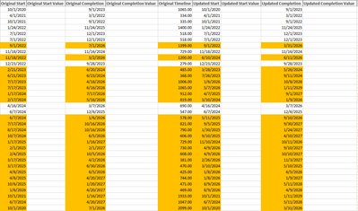
I'm trying to get my date(s) to have correlated values and then use a reference cell to see what the assigned value should be. Please see information below as my example:
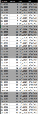
I want to use the values in the columns "Original Start", "Original Completion", "Updated Start", and "Updated Completion" as the inputs for the formula, but checking against this table:
So if the dates in their respective columns fall within any of the ranges in the table above, it assigns the cell the value within the table.
Anyone know how to accomplish this? Thank you!
- Mark as New
- Bookmark
- Subscribe
- Mute
- Subscribe to RSS Feed
- Permalink
- Report Inappropriate Content
Jul 12 2022 09:27 AM
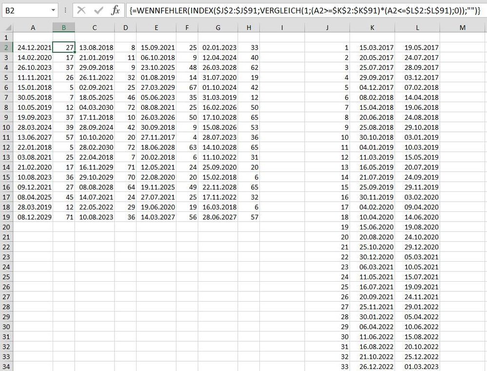
Solution=IFERROR(INDEX($J$2:$J$91,MATCH(1,(A2>=$K$2:$K$91)*(A2<=$L$2:$L$91),0)),"")Maybe with this formula in cell B2. Enter the formula with ctrl+shift+enter if you don't work with Office365 or 2021.
=IFERROR(INDEX($J$2:$J$91,MATCH(1,(C2>=$K$2:$K$91)*(C2<=$L$2:$L$91),0)),"")This is the formula in cell D2 in the example.
- Mark as New
- Bookmark
- Subscribe
- Mute
- Subscribe to RSS Feed
- Permalink
- Report Inappropriate Content
Jul 12 2022 10:18 AM
Accepted Solutions
- Mark as New
- Bookmark
- Subscribe
- Mute
- Subscribe to RSS Feed
- Permalink
- Report Inappropriate Content
Jul 12 2022 09:27 AM
Solution=IFERROR(INDEX($J$2:$J$91,MATCH(1,(A2>=$K$2:$K$91)*(A2<=$L$2:$L$91),0)),"")Maybe with this formula in cell B2. Enter the formula with ctrl+shift+enter if you don't work with Office365 or 2021.
=IFERROR(INDEX($J$2:$J$91,MATCH(1,(C2>=$K$2:$K$91)*(C2<=$L$2:$L$91),0)),"")This is the formula in cell D2 in the example.


