How can I filter out rows that have duplicate values in adjacent columns?

[C_T_M_81]

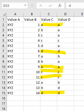
I am trying to filter out rows with duplicate values that appear in adjacent columns.

Full disclosure, its been years since I used Excel in any meaningful way.  Any help is much appreciated.

[#2]

@C_T_M_81 

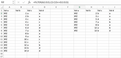
For your example, this function does it: =FILTER(A2:D15,C2:C15<>D2:D15)

I've attached a sample spreadsheet. The formula appears in cell G2; the results fill all the adjacent rows and columns.

(You missed the fourth row in your example, by the way.)

[#3 · Accepted solution]

@C_T_M_81 

You may create a helper column (say in column E) with the following formula...

=C2=D2

This formula will return TRUE when values in columns C and D are the same and FALSE if they are different and then you may apply the Filter and choose TRUE or FALSE as per your requirement.

Please refer to the attached with formula in place.

[#4]

There are couple of ways to go about this. IF you want to filter the existing table I would suggest that you add a helper column and check for duplicates and filter using that column. There are a few ways to do that. 1) you could (and should ) format that data as a table (home->format as a table) and then in the new column you type "=" and then click on the corresponding cell in column C and then "=" and then click corresponding cell in D. What should be typed is something like: =[@[Value C]] = [@[Value D]]. 2) you could type =C2:C15=D2:D15 and assuming you have Excel 365 you will get a column of True/False. Then you goto to DATA menu and click on the Filter to turn on the quick filters 3) if you don't have excel 365 you type =C2=D2 and then fill down. and again you have to turn on the filters Alternatively you could create a new table showing only the filtered results. Assuming you have excel 365 you could type: =FILTER(A1:D15, (C1:C15=D1:D15)+(ROW(A1:A15)=1)) note that ROW(...)=1 is just to copy/show the header row in the new table. again I would recommend you format the data as a table and use table references so it grows and shrinks with the table you don't have to mess with the formula later on.

[#5]

I am having trouble implementing this. I already have a formula active and am not sure which cell to insert the filter in. The sheet i am working on is a large one.  Over 14k rows.

[#6]

That did the trick.

[#7]

Thank you everyone for the input. Very much appreciated.

[#8]

@C_T_M_81 

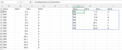
You need FILTER() function by comparing Column C and Column D like-

=FILTER(A2:D15,C2:C15=D2:D15)