- Home
- Microsoft 365
- Excel
- how can I automatically highlight cells used in a formula on another sheet
how can I automatically highlight cells used in a formula on another sheet
- Subscribe to RSS Feed
- Mark Discussion as New
- Mark Discussion as Read
- Pin this Discussion for Current User
- Bookmark
- Subscribe
- Printer Friendly Page
- Mark as New
- Bookmark
- Subscribe
- Mute
- Subscribe to RSS Feed
- Permalink
- Report Inappropriate Content
Apr 27 2023 09:42 AM
I am trying to determine if I can automatically highlight cells used in a formula on another sheet. Is this possible using conditional formatting or another way?
Here is the scenario.
One sheet tallies all expenses by vendor or category for the month by sumifs that look for a few criteria, including the vendor name.
Here's the sheet that tallies by vendor

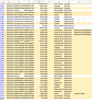
Here is the sheet with the transactions, I have been highlighting them yellow manually so I know which transactions are accounted for on the tally sheet.

Because I have hundreds of transactions a month, with many transactions per vendor and category, I would like to quickly see which transactions have already been added to the vendor tallies so that it's easier to find the expenses that are not reconciled automatically by the formula.
- Mark as New
- Bookmark
- Subscribe
- Mute
- Subscribe to RSS Feed
- Permalink
- Report Inappropriate Content
Apr 27 2023 11:28 AM
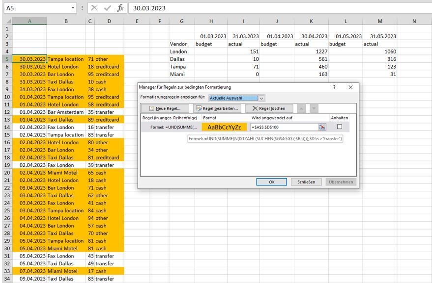
I assume that all dates (months from the first to the last day) are included in the sheet that tallies the vendor. Therefore i've set up a rule for conditional formatting that checks if any of the vendors is included in the cells in column B and if the payment method in column D is <> transfer. For illustration i've made an example in one sheet.
=AND(SUM(N(ISNUMBER(SEARCH($G$4:$G$7,$B5)))),$D5<>"transfer")
This is the rule for conditional formatting in the example. If there are more vendors (4 in the example) than you have to adapt the range in the rule for conditional formatting from $G$4:$G$7 to e.g $G$4:$G$25.
=$A$5:$D$100
This is the range the conditional formatting currently applies to. It can be adapted as required.
=IF(ISODD(COLUMN()),SUMIFS($C$5:$C$100,$A$5:$A$100,">="&G$2,$A$5:$A$100,"<="&H$2,$B$5:$B$100,"*"&$G4&"*",$D$5:$D$100,"<>transfer"),"")
This is the formula in cell H4 which is filled across range H4:M7.
