Hot to capture Slicer selected value from formula?

[Krishnan1989]

Hi @Riny_van_Eekelen/ @L z. ,

I'm using Slicer with non-pivot table. I need to show my slicer selected item/items on another cell. Please provide me any workaround/solution for my problem.

Thank you.

[#2]

@Krishnan1989 

You can use the GETPIVOTDATA function in a formula to capture the selected value from a slicer. However, since you are using a non-pivot table, you will need to use a different approach.

One workaround is to create a helper column in your data range that captures the slicer selection using the IF and COUNTIF functions. Here's how:

1. In a new column next to your data, enter the following formula in the first row: =IF(COUNTIF(slicer_range, data_cell)=1, data_cell, "")

2. Replace "slicer_range" with the range of cells that your slicer controls, and "data_cell" with the cell in your data range that corresponds to the slicer selection.

3. Copy the formula down to all rows in your data range.

4. Finally, in another cell, use the CONCATENATE or TEXTJOIN function to concatenate all non-blank cells in the helper column, which will give you the slicer selection.

Here's an example formula: =TEXTJOIN(", ", TRUE, helper_column_range)

Replace "helper_column_range" with the range of cells that contain your helper column.

Note that this workaround assumes that your data range has unique values for each slicer selection. If your data has duplicate values, this approach may not work as expected.

[#3]

Hi, @Rr_, thank you for the quick response but unfortunately my tables returns duplicate value as well.  To make thinks clear I have created sample of my excel sheet please update your answer in the excel would be great support.

Please use the following link to get the sample of my requirement.

https://docs.google.com/spreadsheets/d/1fWgE0p0u52WahEe-wzg2MhCaMi2coPF-/edit?usp=share_link&ouid=10... 

Many thanks.

[#4]

@Krishnan1989 

Thank you for providing the sample spreadsheet. Based on your sample data, here's a formula you can use in cell B2 to display the selected items from the slicer:

=TEXTJOIN(", ",TRUE,IF($A$2:$A$11=FILTERS!$B$3,$B$2:$B$11,""))

Make sure to enter this formula as an array formula by pressing Ctrl + Shift + Enter after typing it, instead of just Enter. Then, copy the formula down to all rows in your table.

Here's how the formula works:

• FILTERS!$B$3 refers to the cell that contains the selected value in your slicer.
• $A$2:$A$11=FILTERS!$B$3 compares each value in the range A2:A11 with the selected value in the slicer. This will result in an array of TRUE and FALSE values.
• IF($A$2:$A$11=FILTERS!$B$3,$B$2:$B$11,"") returns the corresponding value in column B if the value in column A matches the selected value in the slicer, or an empty string otherwise.
• TEXTJOIN(", ",TRUE,IF($A$2:$A$11=FILTERS!$B$3,$B$2:$B$11,"")) concatenates all non-empty values in the resulting array, separated by a comma and space. The TRUE argument in the TEXTJOIN function tells Excel to ignore empty cells.

I hope this helps! Let me know if you have any further questions.

[#5]

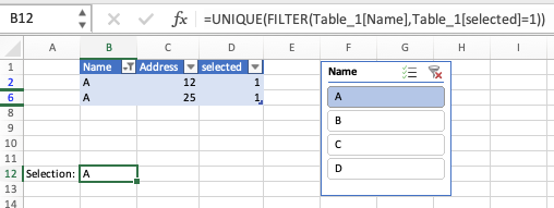
@Krishnan1989 Perhaps the attached file does what you want. Note that I added a helper column to the table that will allow you to filter the table for only visible (i.e. selected) rows.

[#6]

Hi @Riny_van_Eekelen,
1st of all thank you for the reply and I'm using excel 2016 so I can't use the FILTER and UNIQUE function.  

[#7]

Hi @Rr_ ,1st of all thank you for the reply and I'm using excel 2016 so I can't use the FILTER and UNIQUE function.

[#8]

@Krishnan1989 
I'm having out of options if you don't use Filter Function.
I suggest that you download an Filter function Add-In.
Here's the link: Filter Function Add-In