Highlighting a cell based on cell condition

[jaolvera]

Hello, I need help with creating a highlighting condition based on dates. I would want colum M (previously positive) to highlight IF the date in cell T (Test 1 date) is within 60 days of each other. 

[#2]

@jaolvera

Select cells in column M, from M2 down. M2 should be the active cell in the selection.

On the Home tab of the ribbon, click Conditional Formatting > New Rule...
Select 'Use a formula to determine which cells to format'.
Enter the formula

=AND(T2<>"', T2<M2+60)

=AND(T2<>"", T2<M2+60)

Click Format...
Activate the Fill tab.
Select a highlight color.
Click OK, then click OK again.

[#3]

Thank you!
this message popped up? "theres a problem with this formula"

[#4]

@jaolvera 

Do you use comma as decimal separator? If so, use semicolon instead of comma in the formula:

=AND(T2<>""; T2<M2+60)

[#5]

@jaolvera 

Oops, sorry! I had a typo. It should be

=AND(T2<>"", T2<M2+60)

[#6]

the formula worked, but the highlighting condition isnt working when I type in the dates.

[#7]

@Hans Vogelaar

[#8]

@jaolvera 

Could you attach a small sample workbook demonstrating the problem (without sensitive data), or if that is not possible, make it available through OneDrive, Google Drive, Dropbox or similar?

[#9]

@Hans Vogelaar yes I have attached the blank document

[#10]

@jaolvera 

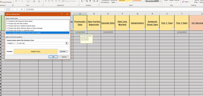
Thanks. The problem is you applied the rule to the entire column $M:$M instead of what I suggested, but the formula still referred to M2 and T2. If the rule applies to the entire column, the formula should refer to M1 and T1.

=AND(T1<>"", T1<M1+60)

See the attached version. (Edited to attach the correct version)

[#11]

thank you so much!