Highlight the minimum value in each row

[Kim Flanagan]

Hi. I'm a complete beginner to Excel and need some help please.
I'm doing a spreadsheet comparing prices from different companies for hundreds of products so I'll have about 10 columns and up to 1000 rows. I want the cheapest price in each row to be highlighted after I input the data.
Could somebody please help me do this? I'll be mainly using Excel android app.
Thank you in advance.

[#2]

Dear Kim,

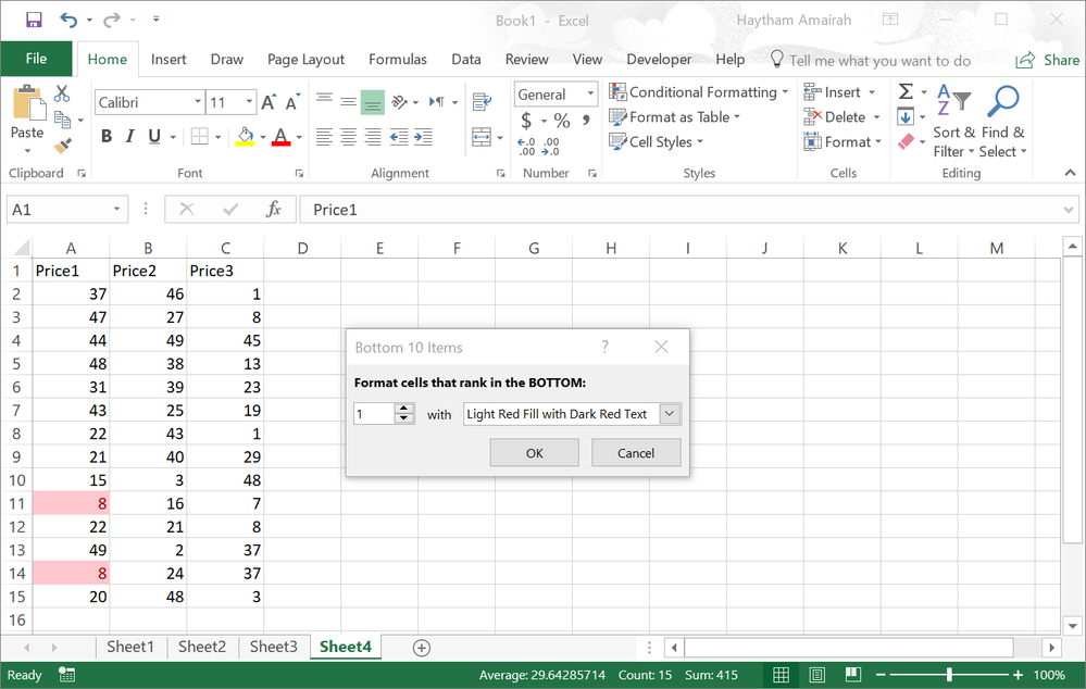
Do the following steps as below screenshot:

1- Highlight the entire first column then go to Home >> Styles >> Conditional Formatting >> Top/Bottom Rules >> Bottom 10 Items...

2- Make the items just 1 item.

3- Select the format that you want, then hit OK.

4- Do the same thing on each column.

[#3]

1. select the first cell in the first row, e.g. Cell A1
2. Home > Conditional Formatting > New Rule > Use a formula to determine which cells to format
3. type the following formula, where $C is the last column 

   =A1=MIN($A1:$C1)

4. click Format button and apply the format you want
5. click OK button (format cell dialog box)
6. click OK button(New Formatting Rule dialog box)
7. Home > Conditional Formatting > Manage Rules
8. You can see your rule, and which cells that it applies to
9. You can change the value in Applies to to apply on all rows.

[#4]

I am sorry, Kim.  I overlooked "be mainly using Excel android app".  I don't have Excel android app. With a search on web, I found this question too.  As of July 2017, conditional formatting is not yet ready in Excel Android App.

[#5]

Can i ask you where someone who is novice in excel, to find such formulas and other useful tips?  Thank you for your response@Willy Lau