Highlight cells on the results of calculated & conditionally formatted cell

[DBrydon]

NOTE: I’m a novice and this wonderful spreadsheet has been developed with the help of members from this forum, so thank you all very much!

Using Excel in Office 365 

I wish to highlight names the same as the highlighted Subtotal cell.

-----------

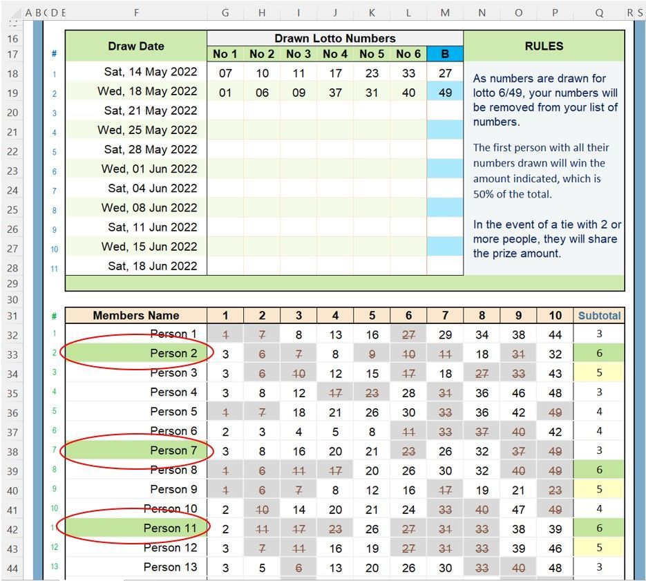
I have a Lotto spreadsheet where drawn lotto numbers are entered in F18:L28

Individual Names are in column F32 and their Lotto Numbers in: G32: P81

The person(s) lotto numbers are subtotaled in: Q32 to Q81

=SUMPRODUCT(--(COUNTIF($G$18:$M$28,$G32:$P32)>0))

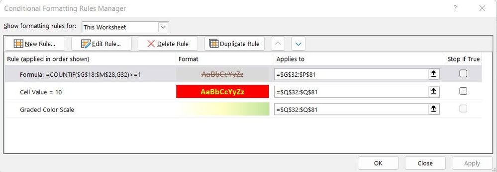
I’ve also applied Conditional formatting to highlight the subtotals to quickly identify those with the most drawn numbers and to ensure duplicate lotto numbers are not counted and grey-out and strike through drawn numbers:

Applies to: =$F$32:$O$81

Formula:   =COUNTIF($F$18:$L$28,F32)>=1

Oops, Person 8 should be highlighted vice Person 7. 

Again, this currently works well, but I would also like to highlight the person(s) name, the same colour as the subtotal field.

Sorry for any confusion in my description, however, I look forward to some guidance.

Cheers,

[#2]

Hi @DBrydon 

Not sure this will work because you don't disclose the Conditional Formatting rule that Applies to Q32:Q81 to highligh Subtotals in green

Edit that Conditional Formatting rule. It currently Applies to: $Q$32:$Q$81

Add ,$F$32:$F$81 at the end:

[#3]

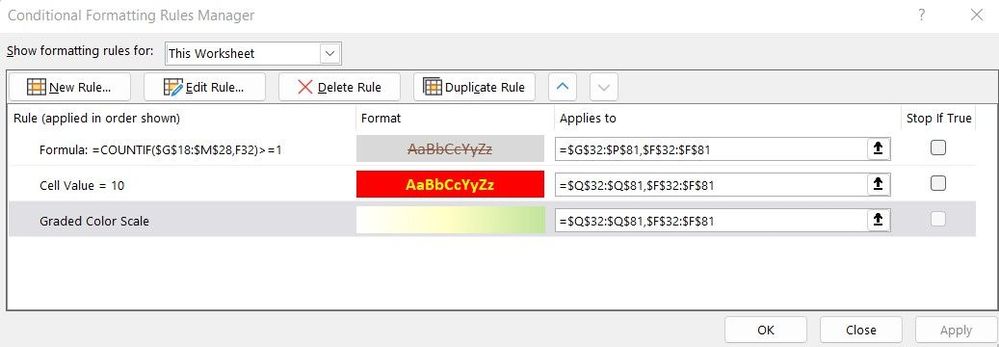
@L z.  Sorry for not providing all the necessary info. I tried to apply your suggestion (hopefully I got that correct :-)), however, no changes occurred. 

I've tried to capture the Conditional Formatting screen for your review.
 

[#4 · Accepted solution]

@DBrydon 

- No reason to change the 1st rule (filling grey) as it doesn't apply to your Subtotal col. Keep it is was

- 2nd rule (filling red) can be adapted to Apply to F32:F81

- 3rd rule (Graded Color Scale), no way. Such rule apply to a single column only and that column must contain numeric values. The only way to go would be to replace this rule by n rules, each matching a number/value (or range of numbers) and filling the corresponding cell(s) with a different color

[#5]

It was just a cosmetic consideration, so I can leave it as is; I shouldn't try to overcomplicate it, or my abilities.
Thank you, as I appreciate your time and guidance.
Cheers.
Dave