Help with this "IFS" statement in office 365

[luigi Pameijer]

I looked up how to write this statement, found a solution on the web (Example 2) see attached image

I typed the exact same information into my spreadsheet using the formula shown.

and get a different result. 

I am using a iMac.

https://support.office.com/en-us/article/IFS-function-36329a26-37b2-467c-972b-4a39bd951d45

Example 2

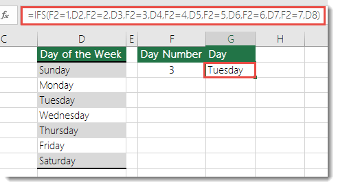
The formula in cell G7 is:

•  =IFS(F2=1,D2,F2=2,D3,F2=3,D4,F2=4,D5,F2=5,D6,F2=6,D7,F2=7,D8)

Why is it that the example has a result of Tuesday but I get #NAME?

Please help

Why is it that I get the result of #NAME? in the cell rateher than the correct result of Tuesday.

I was going to use this formuls to create a formula ( have spelled it out in long hand)

"ifs (the word in this cell is BUTTER) and if (the value in this cell = 2) then insert the value 55, (the word in this cell is CHEESE) and if (the value in this cell = 3) then insert the value 65, (the word in this cell is MILK) and if (the value in this cell = 1) then insert the value 35

The result I get is "#NAME?"

Whats the go?

Luigi

[#2]

Hello Luigi

IFS() is new in Excel 2016 (but only for Office 365 subscribers and in Excel Online).

And for your problem I would suggest a LOOKUP() formula.

[#3]

Or CHOOSE()

[#4]

Hello Detlef,
I am an Office 365 subscriber.
I will try the Lookup option and let you know.
Would it go like this;
=lookup(E8=1,B3="Whey"),15,AND(E8=1,B3="Milk”),15,AND(E8=1,B3="Cheese"),15,AND(E8=1,B3="Butter"),15,AND(E8=1,B3="Meat"),20,AND(E8=1,B3="Bones"),25,AND(E8=1,B3="Grass"),15,AND(E8=1,B3="Water")

[#5]

Hello Sergei,
Detlef suggested Lookup
I will also give Choose a go
Would this formula go something like this;
=choose(E8=1,B3="Whey"),15,AND(E8=1,B3="Milk”),15,AND(E8=1,B3="Cheese"),15,AND(E8=1,B3="Butter"),15,AND(E8=1,B3="Meat"),20,AND(E8=1,B3="Bones"),25,AND(E8=1,B3="Grass"),15,AND(E8=1,B3="Water")

[#6]

---

I am an Office 365 subscriber.

Then IFS() should work.

For the lookup formula create a helper table in E12:F19 with the products in column E and the values in column F. Column E must be sorted in ascending order.

=LOOKUP(B3,$E$12:$F$19)

[#7]

Hello Detlef,

I had another go with the look up formula and still don't get it

See attachemtent

Can you give some pointers

May be I am using the wrong type of formula.

What I am trying to achieve is, from a name in a cell (8 possible options) and a number in another cell (9 options) select a value from a range of cells (in one column) to give a value.

Example if there is water in this cell and the number is 3 then select the number 25

=LOOKUP(U31=3,S31="Bones"),(U31=1,S31="Butter”),(U31=1,S31="Cheese"),(U31=1,S31="Grass"),(U31=1,S31="Meat"),(U31=1,S31="Milk"),(U31=1,S31="Water"),(U31=1,S31="Whey"),25

and then I tried this option too.

=MATCH(U31=3,S31=Bones),(U31=1,S31=Butter),(U31=1,S31=Cheese),(U31=1,S31=Grass),(U31=1,S31=Meat),(U31=1,S31=Milk),(U31=1,S31=Water),(U31=1,S31=Whey),25

[#8]

the choose option is not working either

May be I have the formula wrong or a parameter wrong

Here is a sample attached of what I am trying to achieve

[#9]

Please provide the workbook and not a photo of the workbook.

[#10]

Hello Luigi,

Replying specifically to your BUTTER/CHEESE/MILK formula, the IFS formula should look like this:

=IFS(AND(A1="BUTTER",B1=2),55,AND(A1="CHEESE",B1=3),65,AND(A1="MILK",B1=1),35)

And looks like this in Excel Online:

The formula has been copied down the rows in column C as an example of the result for each combination of values.

The #N/A error occurs as there is no match for the "something is true" of MILK AND 5.

A simple way to avoid this error is to add ' TRUE,"" ' to the end of the formula, like so:

=IFS(AND(A1="BUTTER",B1=2),55,AND(A1="CHEESE",B1=3),65,AND(A1="MILK",B1=1),35,TRUE,"No match")

If each preceeding condition results in FALSE, the final 'condition' is always TRUE and you can display whatever value/text is appropriate.

Hope that helps.

[#11]

Thank you Robert for your assistance.

So far none has effectivley solved the problem.

I am still resulting in the <#NAME?> as the solution to these formula.

It may be a setting in office or excel.

I find that I need to shelve this part of the project for now as I have other pressing tasks.

I will pick it up again in the weeks ahead.

Luigi

[#12]

Detlef, I have attached the complete file as it stands now.

There are a numer of complete as well as incomplete components as you will see.

I was starting a slow process of working out each of the formulas.

It has nothing to do with milk or cheese, they were just easy names that did not need any explanation.

The particular formula I was discussing is on the tab called Pay Calculator where the two conditions are in Cell B3 and E8 with formula resulting in cell F8, H8, J8, L8.

So as the name or value changes in B3 or E8 then so will the values in F8, H8, J8, L8 change.

Thanking you for offering to have a closer look at the situation.

Luigi

www.OodlesofUtils.com

A Game of Choices and Trade Offs

[#13]

Oh my. You are using the wrong quotes.

You are using character 147 (“) instead of character 34 (").

[#14]

Well that is interesting!

Where do I find character 34?

To me 147 looks the same as 34

Is it a specific font type?

[#15]

On my keyboard it's on SHIFT-2.

And to be more precise, you are already using character 34 in the last part of the formula (around No match).

[#16]

How would I know if  i am using 34

The only key on the keyboard that has any similarity to this, is " the key next to the left of the return key.

Also if I am using this key stroke what defines it?

It is getting curious and curiouser!

[#17]

Detlev,

I have copied the quotation marks you mentioned after no match" and then progressivly pasted that into every location for that formula.

The result is the same.

#NAME?

[#18]

Exactly, near return key is straight quote symbol (34) which you shall use in formulas. On Shift+2 is curly quote symbol (147,148) which is for typing text only.

[#19]

Hi Sergei,

I have tried doing that

1 on my imac only 1 key for open Quotation marks " which is [shift"]

I have tried all other keys to no success to find there is only the one "

This is what I have been using all along with the result in the formula being #NAME?

Could this work if I take the quotation marks out all together?

[#20]

No this does not work without the quotation marks.
More testing required.