Help with simple formulas please

[nursekimberley]

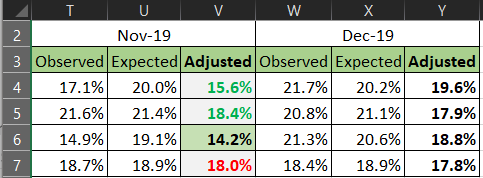
I am not quite successful with this seemingly simple formula.

What I am trying to do (instead of doing it manually) is make the value red if it is higher than the previous months value or make the value green if it is lower that the previous month.

For example, Y4 is > V4 so I want Y4 value to be in red text

For the other formula, Y5 is < V5 so I want Y5 to be in green text

I have tried several different ways and cannot get it to work, any thoughts ple? (I already know how to make the background green when I want it so I do not need that)

[#2]

This can be done with a simple conditional formatting rule.

Highlight the range V5:V7 (V5 is the active cell here) and pick Home => Conditional Formatting => Highlight Cells Rules => Greater than => and then enter V4 as the comparison cell - NO dollar signs. Set your format for green text as the resulting format. Then you can either repeat for Less than, or just manually colour the range red and let the CF rule override that wherever appropriate.

[#3]

@nursekimberley Same as the previous post, but with a picture :)

This can be done through Conditional Formatting with the following settings (picture taken on a Mac, but it's similar on a PC).

Once entered you can "paint" the format by copying it to the next month, as longs it skips two cells each time. 

[#4]

@Riny_van_Eekelen thank you for your input and the person's above.

I have followed the instructions and know how to use the conditional formatting feature but it is cell by cell and I would have to redo that each time i entered one

For instance, i would have to change the cell i am comparing it to each time and when i switch to the next month the same. I am going to attach the full file so you can see. I did Y 4 for both situations but i need to make it copy to all of the values in column Y and then be able to copy the formatiing when i copy the cells for the next month.

Thoughts?

[#5]

@nursekimberley 

Your formatting rules weren't set correctly. Have a look at the attached. I re-did them for you but think I deleted your "Meets benchmark". What's the rule you want to apply there?

[#6 · Accepted solution]

@nursekimberley Could figure out the formatting for the benchmark. Wasn't so difficult after all. With a slight modification, the format is included in the attached file.

Once you are satisfied that a range of cells is properly formatted, you can copy and paste-formats-only to ranges that are to be formatted similarly, provided that you have used the $-signs in the rules correctly.

[#7]

@Riny_van_Eekelen  I will try this now, thank you so much! I will let you know.

[#8]

@Riny_van_Eekelen 

It looks good. the 15% is the benchmark that makes the background green but the other part is opposite.

It is to be red with the percentage went up and green if it went down. I will modify based on what you did and thank you so much!

[#9]

@nursekimberley Great!! Happy to see you can figure out the rest yourself.