Help with Filters

[Banri]

Hi, I am creating a spreadsheet tab called "Curricular Overview" which in turn references two other tabs. "Curriculums" and "Program Data". 

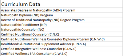
Curriculum Overview is where a dropdown list displays all the types of educational programs are available. 

This is referenced in Program Data
(Curriculum Data is actually Program Data, just forgot to rename it to that)

When Selecting a Program from the Dropdown, It is supposed to grab the Data from Curriculums tab where all the courses to each specific program are stored.

I have added the appropriate filters at the top.
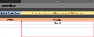
On the Curricular Overview tab, I used the following function in the spot where #CALC! is being displayed in the image below.

=FILTER(Curriculums!B:B,Curriculums!$B:$B = $B$3)

My Issue is that the data is not being pulled from Column B in the Curriculums Tab. Is anyone able to give some assistance? 

[#2]

Hello Banri,

Per Microsoft Support:
"If your dataset has the potential of returning an empty value, then use the 3rd argument ([if_empty]). Otherwise, a #CALC! error will result, as Excel does not currently support empty arrays."

[#3]

@PReagan 

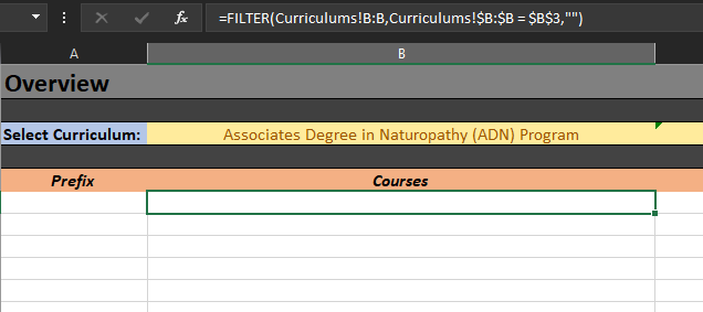
=FILTER(Curriculums!B:B,Curriculums!$B:$B = $B$3,"")

I added this at the end and yes it did removed the #CALC! however it still didnt pull the data from the other tab. I am still really new to all functions & arrays in EXCEL so I am not sure how best to write this.

[#4]

@Banri 

It appears that you may be referencing incorrect data. Be sure that the first array (Curriculums!B:B)

is the array that you want to filter and the second array is the same height or width as the first array. Also be sure that Curriculums!$B:$B contains the value in cell B3. Otherwise, you may be referencing the incorrect column or row.

[#5]

@PReagan 

All the references are correct from the looks of it. I tripled checked everything in those three tabs.
I attached the document if you want to take a look at it.
The Curricular Overview Tab is where the data needs to be pulled from Curriculums.

[#6]

@Banri 

Not sure what you'd like to return into this cell. Perhaps

=XLOOKUP($B$3, 'Program Data'!A:A,'Program Data'!$B:$B, "no data")

which returns

[#7]

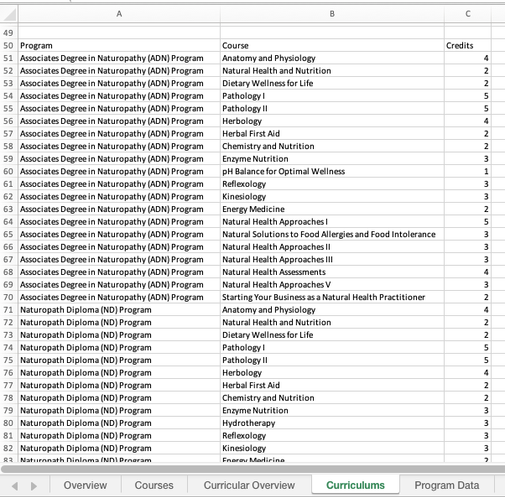
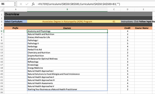
@Banri By looking at your schedule, I believe the original filter formulae were simply referring to the wrong ranges. In addition to that, I'd suggest that you restructure the data in the "Curriculums" sheet, similar to what I have done for the first 2 programs (from row 50 and down).

Then you can more effectively apply the FILTER function to list all the courses and credits belonging to the selected program. In the attached file I used ranges from row 50 to 500, to allow for more programs and courses to be added. But you can adjust these bounds to your real needs. But most importantly is to understand that the first range in the FILTER formula refers to where you want to filter from (in your case, column B holds the course names) and the second range to what you want to filter on (in your case the values in column A should match what you have in B3 on the Overview page). The formula in Column D is similar, though the first range refers to column C in the Curriculums sheet, as this time you want to pick-up the credits. Then, cell C3 in the Overview sums the spilt array in D6.