Help to use a FILTER formula on a FILTER list result

[A_Cannady72]

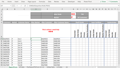
I have enclosed a spreadsheet I’m working building. Cell A7 is a FILTER formula. So that it looks at a table and matches what’s in Cell G2 and it lists all the customers that go with that Sales Node.

Then in columns B & C, I have an Indexed VLookup to match the customer name and market type.

This is where I’m stumped…

I need a formula for Cell D7 that will take the information in columns A-C based on the selection from Cell G3. I have a formula in cell D7, but it exports the result in the cell below it and it doesn’t run through the whole list to create a new list.

My objective is to have the user select a sales node and a market type in cells G2 and G3 and then create a list of customers that fit that criteria. I was successful on the first selection in columns A – C, so I thought I’d replicate the information in columns D – F and just hide A – C before I sent it out.

[#2]

@A_Cannady72 

It seems to me that you might be unaware that you can do the first FILTER with two or more criteria. That might be all you need. For example:

=FILTER({range_to_be_filtered},(criterion1)*(criterion2),"Nothing meets criteria")

Putting an asterisk between the two criteria operates to say "the combination of these criteria" needs to be met, so (If I'm reading your spreadsheet accurately), putting the formula below into Cell A7

=FILTER(EK2:EK11958, (G2=EP2:EP11958)*(G3=ER2:ER11958))

does the trick without the need for a secondary step.

[#3]

@A_Cannady72 

Please view the revised Example and let us know if that is what you need.

[#4]

@A_Cannady72 

All you have to do is fill Sales Node cell G2, and Market cell G3.

then press Data>Refresh All.

Cheers