Help pulling row information from a list using IF

[BriannaYK]

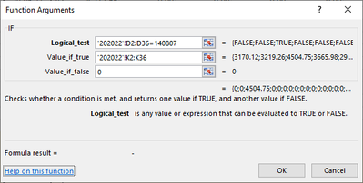
I'm trying to pull information from a row in a separate sheet using if to see if it meets the criteria within a column. e.g. if a cell in column A = 3, I then want it to show the information from column B from the row where it found 3.

In the screenshot I can see there is one TRUE answer where the condition has been met and the 4504.75 that I'm looking for has been identified (below "Value_if_false) but the cell still calculates as zero.

Help! Thanks!

[#2]

@BriannaYK 

I've recently helped someone with a similar issue that has already applied an array formula to pull relevant information into separate tabs in real-time. (Link)

Can you attach your workbook to get a better idea of the data?

[#3]

@adversi Hi, Sorry I'm not sure if I really understand the formula/discussion in the link you provided and I'm afraid I can't attach the document in question 😞 

I was hoping someone could tell me what needs to be added to my formula so that only the cell amount from the row where the condition is true, shows.

[#4]

@BriannaYK 

The reason sending a template would help is to understand the data structure and best formula to apply:

1. Will there be more than one row being pulled by the matched logical test?

2. How many columns of data are in a row?

3. What is the end goal of the workbook - will there only be one tab with final results that you want automatically updated when the condition changes?

The formula will change depending on the answers of the question above, whether it a simple IF can do the job or if an array needs to be created.

[#5]

@BriannaYK 

IMHO, everything works correctly in your case. Function return array of values, if condition is FALSE the value in array is equal to zero, if TRUE - to some number. 

If you are on subscription model, you shall be on Excel with Dynamic Arrays which returns entire such array. The answer will be 0, 0, 4500, 0, etc

Pre-DA Excel will return only first element of such array, e.g. zero. And that's what formula dialogue shows.

If you'd like to return element from third position of the result using the condition TRUE, tat will be another formula. Which one it's better to discuss on your sample.

[#6]

Thanks for your help @SergeiBaklan. Now I understand and yes, I would like only the element with the result using the condition TRUE to be displayed. What formula should I be using for this?

[#7]

@BriannaYK 

Formulas could be different, also depends on your version of Excel. This one shall work in any case

=INDEX('202022'!$K$2:$K$36,MATCH(140807,'202022'!$D$2:$D$36,0))

Better keep lookup value in the cell, let say A1
=INDEX('202022'!$K$2:$K$36,MATCH(A1,'202022'!$D$2:$D$36,0))