- Subscribe to RSS Feed
- Mark Discussion as New
- Mark Discussion as Read
- Pin this Discussion for Current User
- Bookmark
- Subscribe
- Printer Friendly Page
- Mark as New
- Bookmark
- Subscribe
- Mute
- Subscribe to RSS Feed
- Permalink
- Report Inappropriate Content
Jul 27 2021 11:47 AM
I have a very large data file and I am trying to sort but having trouble.
The pivot table looks like this
________________
-91
-100040
-USA
-100200
-USA
-United Kingdom
-123402
-USA
-142389
-USA
-France
etc.
I only want to view trip # (ex:142389) with multiple countries. Trip # with just USA I do not want to see.
Is there any way to do this?
- Labels:
-
Excel
-
Formulas and Functions
- Mark as New
- Bookmark
- Subscribe
- Mute
- Subscribe to RSS Feed
- Permalink
- Report Inappropriate Content
Jul 27 2021 02:16 PM
As variant
For such model
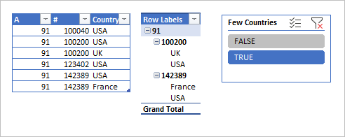
creating PivotTable add data to data model and using DAX add calculated column
=VAR No=[#] VAR qty=CALCULATE(COUNTROWS(Table1), ALL(Table1), Table1[#]=No) RETURN qty>1add filter or slicer on this column.
- Mark as New
- Bookmark
- Subscribe
- Mute
- Subscribe to RSS Feed
- Permalink
- Report Inappropriate Content
Jul 27 2021 03:31 PM
@Sergei Baklan Thank you so much!
I am having trouble implementing this into my own table though :(
As I read about calculated columns, I did not understand them completely.
how did you add your calculated column and then add the slicer?
so far, I have my pivot table set up just how you made yours. I am just unsure how and where to enter the formula to make a calculated column.
I have tried to make a calculated field but i do not think that is the right place, and have tried to enter the formula into the top of the pivot table column but it does not let me enter it. I then thought it was cause the pivot table name is different but changing that did not work either... Thank you for your help this is very advanced for me
- Mark as New
- Bookmark
- Subscribe
- Mute
- Subscribe to RSS Feed
- Permalink
- Report Inappropriate Content
Jul 28 2021 01:16 AM
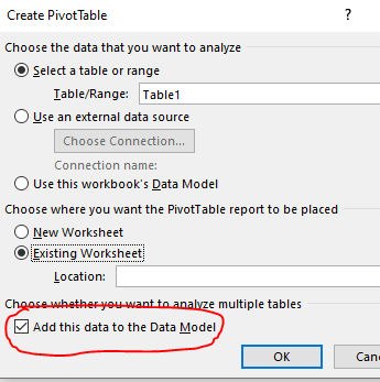
First, creating PivotTable add your data to data model
I assume you are on Windows and on Excel which supports data model.
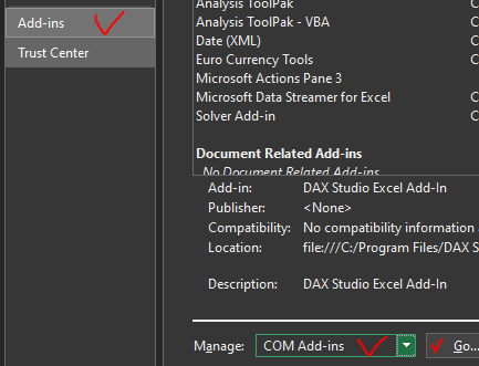
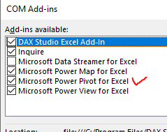
Second, be sure Power Pivot is activated. That is File -> Options -> Add-ins -> COM Add-ins
and here
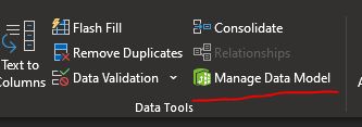
Open it (Data -> Manage data model)
Add new column here to the table
- Mark as New
- Bookmark
- Subscribe
- Mute
- Subscribe to RSS Feed
- Permalink
- Report Inappropriate Content
Jul 28 2021 10:26 AM - edited Jul 28 2021 11:04 AM
Thank you so much for this because I am learning a lot and quite amazed at how much excel can do.
The next issue (Im so sorry... thank you for your time) is
-91
-100040
-USA
-USA
-100200
-USA
-USA
-UK
-123402
-USA
-142389
-USA
-France
-156789
-France
etc
how can I tell excel to differentiate trip # that are USA and another country. If it is just USA or multiple USA I do not want to see it (same if it is just one foreign country or multiple foreign countries). Only trip # that have USA (either once or multiple) AND another country (once or multiple)... I have a feeling it may be an if function but am unsure how to tell excel
***in the image provided, I only want to see trip # such as 101544, 101755, 101783.. trip # such as 101433 with multiple USA or other trip # with multiple Foreign countries and no USA I do not want to see... they have to have both
Thank you again for your help
- Mark as New
- Bookmark
- Subscribe
- Mute
- Subscribe to RSS Feed
- Permalink
- Report Inappropriate Content
Jul 28 2021 01:04 PM
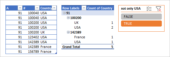
SolutionYou may add column (let say "not only USA") as
=
VAR No = [#]
VAR c = [Country]
VAR withoutUSA =
    CALCULATE (
        COUNTROWS ( Table1 ),
        ALL ( Table1 ),
        Table1[#] = No,
        Table1[Country] <> "USA"
    )
VAR withUSA =
    CALCULATE (
        COUNTROWS ( Table1 ),
        ALL ( Table1 ),
        Table1[#] = No,
        Table1[Country] = "USA"
    )
RETURN
    withoutUSA > 0
        && withUSA > 0
and make filter on it
- Mark as New
- Bookmark
- Subscribe
- Mute
- Subscribe to RSS Feed
- Permalink
- Report Inappropriate Content
Accepted Solutions
- Mark as New
- Bookmark
- Subscribe
- Mute
- Subscribe to RSS Feed
- Permalink
- Report Inappropriate Content
Jul 28 2021 01:04 PM
SolutionYou may add column (let say "not only USA") as
=
VAR No = [#]
VAR c = [Country]
VAR withoutUSA =
    CALCULATE (
        COUNTROWS ( Table1 ),
        ALL ( Table1 ),
        Table1[#] = No,
        Table1[Country] <> "USA"
    )
VAR withUSA =
    CALCULATE (
        COUNTROWS ( Table1 ),
        ALL ( Table1 ),
        Table1[#] = No,
        Table1[Country] = "USA"
    )
RETURN
    withoutUSA > 0
        && withUSA > 0
and make filter on it
