Help on lookup from a list and then display result based on content

[Jimbobmcwalton]

Good morning All,

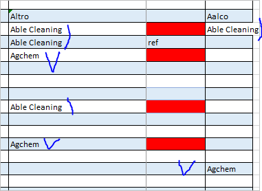
I am trying to get Excel to look at a list from column AC and then if the name is in the list and also in column E (inputted from a drop down list) it colours the cell in column G red.  If the name in column E isn't in column AC then I would like the cell in column G to display "No P/O Req" 

Also, once something is then put into column G I would like the cell to no longer be red.

We are trying to get our worksheet to display a red cell when a customer requires a purchase order number and not be red when we enter a purchase order number hence leaving a visible guide as to which jobs need purchase order numbers in them.   

If anyone can advise the best formula to use for this that would be most appreciated - I have attached the sheet I am using 

Thank you 

Jim  

[#2]

@Jimbobmcwalton 

That's not out of the box function, perhaps some VBA macro you've seen somewhere. But you don't need it, just re-use conditional formatting logic. Count could be calculated as

=SUM(COUNTIFS(Table4[Account],Table4[Column2],Table4[PO / Ref ],""))

it's here

Please note, some texts in Accounts used for data validation have extra spaces, e.g. "Aalco " instead of "Aalco", thus don't match. Please take care and clean your real data.

[#3]

@Sergei Baklan 

You have done it again !   Thank you - works perfectly :) 

[#4]

@Jimbobmcwalton , glad to help

[#5]

@Sergei Baklan 

Hi Sergei,

Would you know why two names now not in column AC are making the cells in column G turn red ?

Seems to be only 2 that are doing this - I have checked the whole of column AC even for text in white or something but cant see anything.

Any ideas?

[#6]

@Jimbobmcwalton 

Could you please give some sample? For the file we discussed here it works correctly