Help - Find the 2nd match using Xlookup

[JMunoz4]

Is there a way using XLookup to return the 2nd (or 3rd, or 4th, or whatever) match in the lookup value? I'm also trying to use as few helper columns as I can. Otherwise I'd just use the VLookup function.

My task is to look through purchase orders and create a pivot table that broke down how much of each material was used. When I created the table I didn't know that there could be multiple instances of the same material in each purchase order.

Here's an example of what I'm looking at.

Order 1   Material 1   6 Inches

Order 1   Material 1   6 Inches

Order 1   Material 2   32 Inches

Order 1   Material 3   41 Inches

Order 2   Material 1   7 Inches

Order 2   Material 2   33 Inches

Order 2   Material 2   33 Inches

Order 2   Material 3   41 Inches

Order 2   Material 4   16 Inches

Order 3   Material 1   6 Inches

Order 3   Material 1   6 Inches

Order 3   Material 1   8 Inches

Order 3   Material 2   19 Inches

Order 3   Material 3   40 Inches

Order 3   Material 3   41 Inches

Order 3   Material 4   18 Inches

[#2]

@JMunoz4 Are you sure a regular pivot table won't work? See attached.

If this does not make sense, how exactly would you want to summarise the data?

[#3]

@JMunoz4 

If you wish to list multiple matches FILTER would be a more appropriate function

= FILTER(Orders[[Material]:[Size]], Orders[Order]=Selected)

If you wish to aggregate similar values then that could be a Pivot Table or SUMIFS/COUNTIFS combined with UNIQUE to identify the possibilities.

[#4]

@Riny_van_Eekelen 

Thank you. I am still curious if XLOOKUP can return the nth match in an array. But now that you mention it, redoing the pivot table would be the best way to display what I'm looking for. I don't have much experience with pivot tables so I sorta reverse engineered one from a similar worksheet.

[#5]

@JMunoz4 

It seems possible. Here is an example.

Formula:

=XLOOKUP(
   F2:F5&H1,
   B1:B16&
      SORTBY(
        SEQUENCE(ROWS(B1:B16),1,2)-MATCH(SORT(B1:B16),SORT(B1:B16),0),
        SORTBY(SEQUENCE(ROWS(B1:B16),1,2),B1:B16,1),1
      ),
   C1:C16
)

Source

[#6]

@excelmee
Would this formula need to be revised to find the nth result when using only one lookup value (F2)? I tried the formula you posted and it didn't work in such a case.

[#7]

@LSpurchasing 

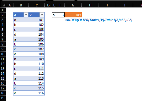
If you need nth occurrence, the easiest way is based on what @Peter Bartholomew  suggested

[#8]

@Sergei Baklan 

Perfect!  Thanks

[#9]

@LSpurchasing You just need to change F2:F5&H1 to F2&H1.

If you have a single search key better follow the Index + Filter combo.

[#10]

Thank you @Peter Bartholomew  and @Sergei Baklan saved me a ton of time today. Appreciate this community. 

[#11]

@MobileTim , glad to know this forum helped