Help and Old Man Out Please

[JackP326]

I have attached a worksheet that illustrates the two problems that I am having.  The spreadsheet has comments in cells that shows what I am trying to accomplish.  The spreadsheet is just an example of the real life spreadsheet which is several thousands of rows (and more to be added) and 60 columns that need to do this equation.  Feel free to add as many columns as needed to solve the problem but the solution needs to be contained in each row.

My Grandson ( the smartest person in my family) couldn't solve the problem and he is my only resource.  Any help would be greatly appreciated.

Thanks in Advance

Jack

[#2]

@JackP326 

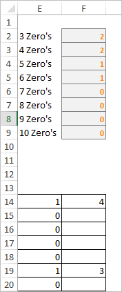
Jack, variant of calculations is in next columns:

In E14

=--(A14=1)

in F14

=IFNA(IF(E14,MATCH(1,INDEX(E:E,ROW()+1):E$1000,0)-1,""),"")

and drag them down till end of range.

In F2

=COUNTIF(F$14:$F$1000,LEFT(E2,SEARCH(" ",E2)-1))

and also drag it down.

[#3]

@Sergei Baklan 

Sergie

Thank you so much for your quick response.  Let me ask is it possible for the calculation to be at the bottom as an example have the 4 that I had in C14 be located at C19?  In addition when I tried your solution for F2 and I dragged down it didn’t result in any totals is just put 0 in the cell.

[#4]

@JackP326 

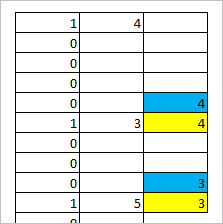
Let me clarify - you'd like count of zeroes against next 1 (yellow) or against last zero (blue) in the series?

Formula in F2 works on column F, not on column C, perhaps you didn't adjust it.

[#5]

@Sergei Baklan 

Next to1 the yellow example

I did try in F column and all that i get is zero's

[#6]

@JackP326 

Please find it in the Sheet2 of the attached file.

[#7]

@Sergei Baklan 

Sergi,

You are a Rock Star.  Thanks so much for your help

[#8]

@JackP326 , you are welcome

[#9]

@Sergei Baklan 

Sergei,

I have one last issue.  I don't  know the formula to accomplish my example in the E Column Rows 20-63 of the attached worksheet.  I thought I was going to be able adapt the other formula to use here but it is beyond my skills.  Any help would be greatly appreciated.  I have highlighted the area in yellow that contains the issue

Jack

[#10]

@JackP326 

Jack, sorry, but  I didn't catch the logic.

- why first number appears in E26, next series starts at E34, etc

- why it is nothing between E41 and E52

- why zero is in E30, E36 but not in E41, E63?

Perhaps other similar question, for me general logic is not clear.

[#11]

@Sergei Baklan 

I see some of my logic errors let me make corrections and I will forward to you a revised spreadsheet.

[#12]

@JackP326 

I have seen the error of my ways and hopefully this example will clear things up.  

[#13]

@JackP326 

Thank you, I'll check bit later

[#14]

@JackP326 

I'd suggest to add helper column D

with formula

=IF($B21,1-$E$13,D21+1)

and next column E will be as

=IF(
      (IF($B21,1-$E$13,D21+1) <1) + (IF($B21,1-$E$13,D21+1) >$E$15),
      0,
      INDEX($E$2:$E$11,IF($B21,1-$E$13,D21+1))
)

formulas start from row 22, drag them down till end of the range.

I forgot to adjust these formulas for very first row (#21 here), thus to simplify let consider it as helper row in which A21 and B21 are always equal to 1.

[#15]

@Sergei Baklan 

Sergei,

Once again thank you so  much.  If you would be so inclined please email at jack@phelanmail.com

I would like to tell you something that I prefer not to do on a public forum.

Jack