Having a text formula update automatically across multiple sheets when I add additional information

[johnsboxftm]

Hello, all.

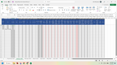
So I currently have an IFS formula written into cells C3:C30.  It's set up so that if I type in a city name it puts in the tax rate so I don't have to type it out constantly for each city.

=IFS(B3="Chagrin Falls", 8%, B3="Berea", 8%, B3="Warren", 6.75%, B3="Etna, PA", 7%, B3="Elyria",6.5%, B3="Cleveland", 8%, B3="West Salem", 6.5%, B3="Hudson", 6.75%, B3="Toledo", 7.75%, B3="Wooster", 6.5%, B3="Brooklyn", 8%, B3="Streetsboro", 7%, B3="Bedford Heights", 8%, B3="Norton", 6.75%, B3="Canton", 6.5%, B3="Northfield", 6.75%, B3="East Cleveland", 8%, B3="Shaker Heights", 8%, B3="Avon", 6.5%, B3="Ashtabula", 6.75%, B3="Kent", 7%, B3="Bratenahl", 8%, B3="Hinckley", 6.75%, B3="North Royalton", 8%, B3="Medina", 6.75%, B3="Wadsworth", 6.75%, B3="Cuyahoga Falls", 6.75%, B3="Mentor", 7.25%, B3="Warrensville Heights", 6.5%, B3="Bridgeport", 7%, B3="Bedford Heights", 8%, B3="Broadview Heights", 8%, B3="Lakewood", 8%, B3="Eastlake", 7.25%, B3="Akron", 6.75%, B3="Lorain", 6.5%, B3="Highland Heights", 8%, TRUE, "Enter Rate")

I occasionally have to update the formula with new cities our company hasn't conducted business in before.  When I add the city in, is there a way for when I make these occasional additions that they would automatically update across the rest of the sheets (February 2023, March 2023 and so on)?  This way I don't have to manually copy and paste the new IFS formula to each sheet individually then drag them down, etc.

Thank you and I appreciate your help

J

[#2]

Don't hard code the values in the formula, create a table of cities and percentages, then lookup the % to use using the city name as a key...

[#3]

Hi @johnsboxftm ,

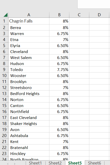
If you have the option to create an additional table to store all of the cities and tax rates, you can use the VLOOKUP instead of the IFS. In the table below, I stored some cities and tax rates in a separated sheet:

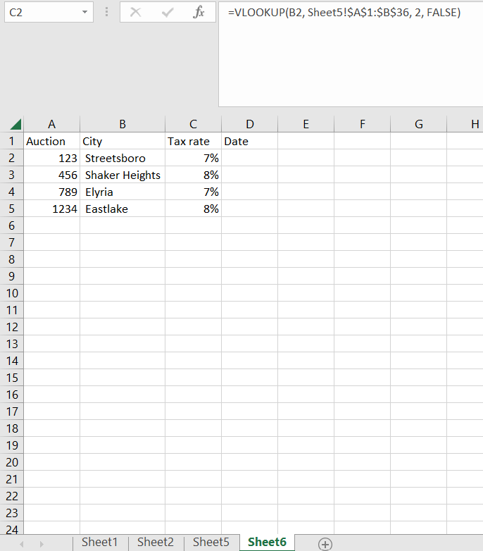
Then, in your table you just apply this formula in the Tax Rate column: =VLOOKUP(B2, Sheet5!$A$1:$B$36, 2, FALSE). It will looks like this:

You just have to take the following precautions:

1. When you add a new city to the list, make sure to expand the range of the table used in VLOOKUP formula;

2. The city name (the look up value) have to be on the left side of the table where you store the tax rates;

3. Keep the last argument as FALSE.

If this answer does not solve your problem, please let me know.

[#4]

How do I do that?

[#5]

Thank you for this, I will implement it shortly, If I may ask, how did you transfer the information from my IFS formula to the columns on sheet 5 when you made the table? Did you have to enter them each individually or is there a way to import that info?

[#6]

@johnsboxftm here is a file with the example. You will have to create a separated table to store the cities/tax rates (Sheet1, in the attached file), and then you just refer to it with your main table, by using the VLOOKUP formula.

For the VLOOKUP, you will use the following parameters:

City - The city that you want to find in the cities/taxes table (in the attached file, Sheet2, column B)

Range - The range of the cities/taxes table (in the attached file, Sheet1, A1:B36);

ColNumber - The number of the column, in Range, that you want to return the information, it means the tax rate (in attached file, Sheet1, column b)

RangeLookup - For your use case, set this parameter as false.

So you will build the formula in your file like this: VLOOKUP(City, Range, ColNumber, FALSE). 

Let me know if you need any additional help with it. 

[#7]

1. I just copied your formula and pasted in a cell;
2. After, used the Text to Columns feature, in data tab of the ribbon, to separate it into columns, using comma as separator;
3. Then I copied the whole row and pasted in a cell, using the Transpose paste option, transforming it into a column with cities and tax rates;
4. Then I filtered all of the results by "%", copied it and pasted somewhere else;
5. After have the tax rates properly saved, just deleted all of them from the column and removed the duplicates to delete the blank cells and let only the city names;
6. Finally, I pasted the tax rates (that I saved somewhere else) on the side of the cities.

You can find this table in the file that I sent you in the last comment. In any case, double check it to make sure that I didn't messed with some tax rate in this process :)