- Home
- Microsoft 365
- Excel
- Re: Grouping TRUE/FALSE answers into a single cell.
Grouping TRUE/FALSE answers into a single cell.
- Subscribe to RSS Feed
- Mark Discussion as New
- Mark Discussion as Read
- Pin this Discussion for Current User
- Bookmark
- Subscribe
- Printer Friendly Page
- Mark as New
- Bookmark
- Subscribe
- Mute
- Subscribe to RSS Feed
- Permalink
- Report Inappropriate Content
Sep 27 2022 09:02 PM
Hi all,
To preface, I am an Excel novice, so I apologise in advance for my ignorance.
What I'm looking to do is create a tool wherin employees (contact centre) can select a checkbox of what they have completed in a call interaction and then based on the TRUE/FALSE answers of the checkboxes, it generates notes that they can copy/paste into other software.
As an example: during the call, the agent updates a phone number, and email, and resets an online password. They would select the three checkboxes relevant to this, then excel would spit out notes like:
-Updated the member's phone number.
-Updated the member's email address.
-Reset the online password.
What I have so far is all of the options and a checkbox for each option which generates a T/F result. I am also able to change the T/F answer to spit out the desired notes. The problem lies in that it is not copy/paste friendly, as the cells are far apart.
Is there any way to, for example, check which options are T/F and group only the TRUE answers together in one cell?
Please let me know if you need any clarification on anything.
Thanks in advance.
- Labels:
-
Excel
-
Macros and VBA
- Mark as New
- Bookmark
- Subscribe
- Mute
- Subscribe to RSS Feed
- Permalink
- Report Inappropriate Content
Sep 28 2022 12:46 AM
could you please provide a sample of your file? This would make it easier to see what you have done already (and how), otherwise we would need to spent efforts on things that already exist.
The other question:
What Excel version do you use? This is important for proposing a proper solution.
- Mark as New
- Bookmark
- Subscribe
- Mute
- Subscribe to RSS Feed
- Permalink
- Report Inappropriate Content
Sep 28 2022 03:55 PM
@Martin_Weiss Hi Martin,
Here is the link to the spreadsheet. I am working on Excel 2016.
Hope that helps. Let me know if you need anything else.
Regards,
Ben
- Mark as New
- Bookmark
- Subscribe
- Mute
- Subscribe to RSS Feed
- Permalink
- Report Inappropriate Content
Sep 29 2022 12:32 AM
Solution
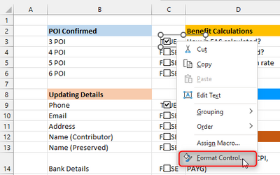
thanks for the file. First of all, you need to link every checkbox to a cell. Right-click on the ceckbox and select "Format control..."
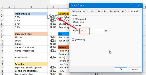
Then link it to the cell right below the checkbox:
The cell will get the value TRUE or FALSE based on wether the checkbox is checked or unchecked.
(You can make the TRUE/FALSE values invisible later by changing the font color to white or with a user defined number format)
Last thing is to concatenate all values in the column B, D and E that have a TRUE statement in the cell right to them.
Unfortunately, this is going to be a very long formula in Excel 2016. I just did it in the attached file for column B, so you can get the idea:
=IF(C3=TRUE,B3,"")&IF(C4=TRUE,", "&B4,"")&IF(C5=TRUE,", "&B5,"")&IF(C6=TRUE,", "&B6,"")&IF(C9=TRUE,", "&B9,"")&IF(C10=TRUE,", "&B10,"")&IF(C11=TRUE,", "&B11,"")&IF(C12=TRUE,", "&B12,"")&IF(C13=TRUE,", "&B13,"")&IF(C14=TRUE,", "&B14,"")&IF(C15=TRUE,", "&B15,"")&IF(C16=TRUE,", "&B16,"")&IF(C17=TRUE,", "&B17,"")&IF(C18=TRUE,", "&B18,"")&IF(C19=TRUE,", "&B19,"")&IF(C20=TRUE,", "&B20,"")&IF(C21=TRUE,", "&B21,"")&IF(C22=TRUE,", "&B22,"")&IF(C23=TRUE,", "&B23,"")&IF(C24=TRUE,", "&B24,"")&IF(C25=TRUE,", "&B25,"")&IF(C26=TRUE,", "&B26,"")&IF(C29=TRUE,", "&B29,"")&IF(C30=TRUE,", "&B30,"")&IF(C31=TRUE,", "&B31,"")
There might be more sophisticated solutions, but this was the only one I can think of at the moment.
Just for information: With Excel in Microsoft 365, you get the same result with just this simple formula:
=TEXTJOIN(", ",TRUE,FILTER(B3:B31,C3:C31=TRUE))
I have attached your sample file where I have prepared it for columns B/C.
Hope this helps.
Accepted Solutions
- Mark as New
- Bookmark
- Subscribe
- Mute
- Subscribe to RSS Feed
- Permalink
- Report Inappropriate Content
Sep 29 2022 12:32 AM
Solution
thanks for the file. First of all, you need to link every checkbox to a cell. Right-click on the ceckbox and select "Format control..."
Then link it to the cell right below the checkbox:
The cell will get the value TRUE or FALSE based on wether the checkbox is checked or unchecked.
(You can make the TRUE/FALSE values invisible later by changing the font color to white or with a user defined number format)
Last thing is to concatenate all values in the column B, D and E that have a TRUE statement in the cell right to them.
Unfortunately, this is going to be a very long formula in Excel 2016. I just did it in the attached file for column B, so you can get the idea:
=IF(C3=TRUE,B3,"")&IF(C4=TRUE,", "&B4,"")&IF(C5=TRUE,", "&B5,"")&IF(C6=TRUE,", "&B6,"")&IF(C9=TRUE,", "&B9,"")&IF(C10=TRUE,", "&B10,"")&IF(C11=TRUE,", "&B11,"")&IF(C12=TRUE,", "&B12,"")&IF(C13=TRUE,", "&B13,"")&IF(C14=TRUE,", "&B14,"")&IF(C15=TRUE,", "&B15,"")&IF(C16=TRUE,", "&B16,"")&IF(C17=TRUE,", "&B17,"")&IF(C18=TRUE,", "&B18,"")&IF(C19=TRUE,", "&B19,"")&IF(C20=TRUE,", "&B20,"")&IF(C21=TRUE,", "&B21,"")&IF(C22=TRUE,", "&B22,"")&IF(C23=TRUE,", "&B23,"")&IF(C24=TRUE,", "&B24,"")&IF(C25=TRUE,", "&B25,"")&IF(C26=TRUE,", "&B26,"")&IF(C29=TRUE,", "&B29,"")&IF(C30=TRUE,", "&B30,"")&IF(C31=TRUE,", "&B31,"")
There might be more sophisticated solutions, but this was the only one I can think of at the moment.
Just for information: With Excel in Microsoft 365, you get the same result with just this simple formula:
=TEXTJOIN(", ",TRUE,FILTER(B3:B31,C3:C31=TRUE))
I have attached your sample file where I have prepared it for columns B/C.
Hope this helps.


