- Home
- Microsoft 365
- Excel
- Re: Gantt chart - Pull start/end dates
Gantt chart - Pull start/end dates
- Subscribe to RSS Feed
- Mark Discussion as New
- Mark Discussion as Read
- Pin this Discussion for Current User
- Bookmark
- Subscribe
- Printer Friendly Page
- Mark as New
- Bookmark
- Subscribe
- Mute
- Subscribe to RSS Feed
- Permalink
- Report Inappropriate Content
Jul 13 2020 08:24 PM
I am trying to find a way to import Gantt charts from excel into Monday.com so that I can have the tasks and date ranges. I am trying to find a way (formula/programming) so that for each row I can pull the start date (first green cell for the row) and end date (first cell after green minus 3 days or last green cell plus 4 days to capture Friday being the last day for the project) from the headers. I have no idea if this is possible or how I would go about doing this. I am including a picture of what I am talking about. I have manually entered the date ranges in column V (preferred) or the start and end dates in separate columns X&Y. This is what I am trying to achieve.
Can anyone help?
- Labels:
-
Excel
- Mark as New
- Bookmark
- Subscribe
- Mute
- Subscribe to RSS Feed
- Permalink
- Report Inappropriate Content
- Mark as New
- Bookmark
- Subscribe
- Mute
- Subscribe to RSS Feed
- Permalink
- Report Inappropriate Content
Jul 14 2020 09:31 AM - edited Jul 14 2020 09:35 AM
Solution
This will be easier if you have some values in the colored cells.
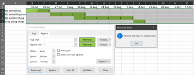
So, first select the range that contains the colored cells, then use Ctrl+H to find and replace blank green cells with green cells containing a 1. Like this:
(p.s. I had no idea until today that this was even possible, so TIL I guess!)
After that, you can use XLOOKUP using the default first-to-last search to return the start date:
=XLOOKUP(1,$B2:$O2,$B$1:$O$1,"")
This will look in cells B2 to O2 for a 1 and return the value from row 1 in the same column (i.e. the week commencing date).
And using a last-to-first search to return the end week, then add 4 to get the Friday of that week:
=XLOOKUP(1,$B2:$O2,$B$1:$O$1,"",0,-1)+4
This will look backwards from cell O2 to B2 for the first 1 it finds and likewise return the week commencing date from row 1, then add 4 to that.
Please see attached example.
If you want to create a single column with the date range, you can use this:
=TEXT(XLOOKUP(1,$B2:$O2,$B$1:$O$1,""),"m/dd")&"-"&TEXT(XLOOKUP(1,$B2:$O2,$B$1:$O$1,"",0,-1)+4,"m/dd")- Mark as New
- Bookmark
- Subscribe
- Mute
- Subscribe to RSS Feed
- Permalink
- Report Inappropriate Content
Jul 14 2020 09:12 PM
@OwenPrice Perfect! Thank you so much. And I'm glad you were able to learn something, too :)
Accepted Solutions
- Mark as New
- Bookmark
- Subscribe
- Mute
- Subscribe to RSS Feed
- Permalink
- Report Inappropriate Content
Jul 14 2020 09:31 AM - edited Jul 14 2020 09:35 AM
Solution
This will be easier if you have some values in the colored cells.
So, first select the range that contains the colored cells, then use Ctrl+H to find and replace blank green cells with green cells containing a 1. Like this:
(p.s. I had no idea until today that this was even possible, so TIL I guess!)
After that, you can use XLOOKUP using the default first-to-last search to return the start date:
=XLOOKUP(1,$B2:$O2,$B$1:$O$1,"")
This will look in cells B2 to O2 for a 1 and return the value from row 1 in the same column (i.e. the week commencing date).
And using a last-to-first search to return the end week, then add 4 to get the Friday of that week:
=XLOOKUP(1,$B2:$O2,$B$1:$O$1,"",0,-1)+4
This will look backwards from cell O2 to B2 for the first 1 it finds and likewise return the week commencing date from row 1, then add 4 to that.
Please see attached example.
If you want to create a single column with the date range, you can use this:
=TEXT(XLOOKUP(1,$B2:$O2,$B$1:$O$1,""),"m/dd")&"-"&TEXT(XLOOKUP(1,$B2:$O2,$B$1:$O$1,"",0,-1)+4,"m/dd")

