Formulas and Functions

[pjukes]

Hello,

I was hoping someone could help me.

I am having trouble attempting to create a formula in my excel spreadsheet.

I would like all the cells in one column to automatically calculate a dollar figure based on numbers entered in an adjacent column.

Example 1: If C6 has a figure between 50.00 & 100.00 D6 should display $1.50

Example 1: If C6 has a figure between 101.00 & 150.00 D6 should display $2.00

Example 1: If C6 has a figure between 151.00 & 200.00 D6 should display $2.50

If there is a formula for this example I would really appreciate any assistance.

Thank you,

Paul

[#2]

@pjukes 

In D6:

=(ROUNDUP(C6/50,0)+1)/2

Does that do what you want?

[#3]

@pjukes 

A minor difference of function but the main difference is that I avoid scalar fill-down formulas when an array formula would do the same job!

[#4]

@Hans Vogelaar 

Hi Hans,

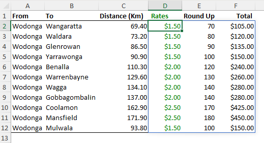
Unfortunately that didn't work, please see below .

From	To	Distance (Klm)	Rates	Round Up	Total
Wodonga	Wangaratta	69.40	$        1.50	70.00	$       105.00
Wodonga	Waldara	73.20	$        1.50	80.00	$       120.00
Wodonga	Glenrowan	86.50	$        1.50	90.00	$       135.00
Wodonga	Yarrawonga	90.90	$        1.50	100.00	$       150.00
Wodonga	Benalla	110.30	$        2.00	120.00	$       240.00
Wodonga	Warrenbayne	129.60	$        2.00	130.00	$       260.00
Wodonga	Wagga	134.10	$        2.00	140.00	$       280.00
Wodonga	Gobbagombalin	137.00	$        2.00	140.00	$       280.00
Wodonga	Coolamon	162.90	$        2.50	170.00	$       425.00
Wodonga	Mansfield	171.90	$        2.50	180.00	$       450.00
Wodonga	Mulwala	93.80	$        1.50	100.00	$       150.00

I need the rate to increase as per the round up total eg: 50.00 - 100.00 = $1.50, 101.00 - 150.00 = $2.00 ect...

[#5 · Accepted solution]

@pjukes 

I pasted your example into a worksheet, then added formulas based on the one in my previous reply.

Sheet 1 is your example, Sheet2 has the formulas. The results appear to be the same.

[#6]

@pjukes 

This problem seems to be changing by the day?  In addition it is not obvious to me what rate should correspond to 100.5 km.  Anyway, to extend my former solution attempt

= LET(
    rates, CEILING.MATH(50 + distance, 50) / 100,
    rndUp, CEILING.MATH(distance, 10),
    HSTACK(rates, rndUp, rates*rndUp)
  )

[#7]

Thank Hans, this formula has done the job. Much appreciated.

[#8]

Thanks Peter, My issue has been solved. Appreciate the assistance.