Formulaic calculation of table rows

[akseeker]

I'm trying to automatically update a chart that only displays the last 30 entries in a large (>600 rows) table.

I can't find a formula like "=NumRows(Table1)" to use in calculating the max number of rows, then with a formula (in the 'choose data' dialog) set the chart range to '=NumRows(Table1)-30:NumRows(Table1), for instance.

Does such an animal exist? Can counting table rows be accomplished without resorting to VB?

Now, I select the chart's value line, the data it's based on is enclosed/highlighted, and I manually move the data targets down a row to only include the last 30 rows; be neat to not have to do that manually.

Thanks!

[#2]

Hi @akseeker,

You seem to referring some custom function NumRows. There is no built-in function.

What i understood you wish to get the last 30 day transaction from the range, Well I can suggest you try building using OFFSET function.. If you still facing issue attach a sample file.

Regards, Faraz Shaikh | MCT, MIE, MOS Master, Excel Expert

If you find the above solution resolved your query don't forget mark as Official Answer to help the other members find it more.

[#3]

If you find the above solution resolved your query don't forget mark as Official Answer to help the other members find it more.

[#4]

@Faraz Shaikh you are correct, I was looking for a function that would return the total number of rows in a table in order to use the offset function. Unless you know the total number of rows in the table, how would you apply the offset function?

So, my question is, how does one (functionally) determine the number of rows in a table?

Thanks

[#5 · Accepted solution]

HI @akseeker 

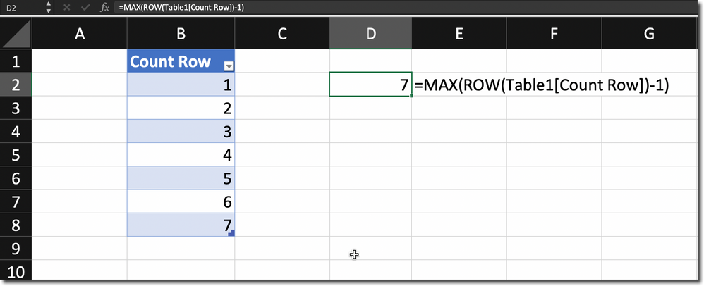
You need to construct array formula, here is how it should work. If you are using office365 with new dynamic arrays calculation engine you can paste the formula straight away

=MAX(ROW(Table1[Count Row])-1)

If not paste the formula and press ctrl + shift + enter 

Regards, Faraz Shaikh | MCT, MIE, MOS Master, Excel Expert

If you find the above solution resolved your query don't forget mark as Official Answer to help the other members find it more

[#6 · Accepted solution]

If you find the above solution resolved your query don't forget mark as Official Answer to help the other members find it more

[#7]

Great answer @Faraz, that worked perfectly, thank you.

PS: I looked in all the drop-down menus I could see on this page, but can't see an obvious way to set the question to 'solved'. I set it to Best Response, but don't see how to set it to 'Official Answer'. How is that accomplished?

[#8]

Thanks @Faraz Shaikh , now the next problem is using that info in the Chart:Data dialog:

(attached a spreadsheet as example)

The formulas currently read =Widgets!$I$71:$I$101 in the Y-Value field, and =Widgets!$A$71:$A$101 in the 'Horizontal (Category) axis labels' field.

I've named the results of the "{=MAX(…)-30}" cell to ChartStartRow (H104), and the result of the {=MAX(…))} to ChartEndRow (H105). I concatenated those into a cell, with the calculated ranges listed out in text format, and named the cells XRange (J104) and YRange (J105).

How do I get that calculation into the X and Y-Values fields in the chart data dialog box? I tried several approaches, but they all resulted in errors. It doesn't appear formulas [e.g. INDIRECT()] are allowed in the Select Data Source fields.

I wanted to avoid VB…

Thanks in advance!