formula

[radial2021]

How do I add 7 rows and then take that information and get the sum of that information in different columns in the 7 rows. Once I have that information I want to be able to copy and paste that information into the cell below it and have the next seven rows added and have the sum of the next 7 rows summed in different columns =IF(COUNT(Data!A2:A8)=7,SUM(BM2:BM8)) looking at this formula this would be the first cell, the second cell should read =if(count(data!A9:A15)=7,sum(BM9:BM15)). I want to be able to copy and paste so each cell below is the next 7 rows summing that group of information. If this is not the correct formula please let me know, I am just trying different options

Thank you

[#2]

@radial2021 

To sum the values in different columns for a range of 7 rows and then copy the formula down for subsequent ranges, you can use the OFFSET function along with the SUM function.

Here's an example formula that you can use:

=SUM(OFFSET(BM2,(ROW()-2)*7,0,7,1))

This formula will start summing at the cell BM2, and then offset by 7 rows for each subsequent range. The ROW() function returns the current row number, so by subtracting 2 (since the formula starts in row 2), multiplying by 7 (since there are 7 rows in each range), and then adding that value to the starting cell reference, the formula will sum the correct range for each subsequent row.

To copy and paste the formula down for subsequent ranges, simply select the cell with the formula, and then drag the fill handle (the small square at the bottom right corner of the cell) down to the next cell where you want to paste the formula. The formula will automatically adjust to sum the next range of 7 rows.

*The formula you provided is correct.

I hope this helps! 

[#3]

@NikolinoDE

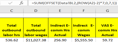
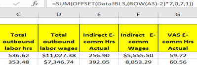
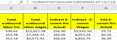
Thank you for the information, I put the new formula and for the first 2 lines it worked by then the 3rd line it skipped 2 rows.  see below (information followed by picture of formula, and then the error

Thank you for your help with this

1/1/2023	$0.00
1/2/2023	$0.00
1/3/2023	$147.97
1/4/2023	$149.09
1/5/2023	$139.85
1/6/2023	$99.71
1/7/2023	$0.00	536.62
1/8/2023	$0.00
1/9/2023	$87.71
1/10/2023	$89.91
1/11/2023	$81.35
1/12/2023	$49.46
1/13/2023	$45.05
1/14/2023	$0.00	353.48
1/15/2023	$0.00
1/16/2023	$0.00
1/17/2023	$77.51
1/18/2023	$69.44
1/19/2023	$39.83
1/20/2023	$36.47
1/21/2023	$0.00	223.25
1/22/2023	$0.00
1/23/2023	$89.91	313.16
1/24/2023	$82.83
1/25/2023	$49.50
1/26/2023	$54.89
1/27/2023	$51.51
1/28/2023	$0.00	328.64

1/1/2023	$0.00
1/2/2023	$0.00
1/3/2023	$147.97
1/4/2023	$149.09
1/5/2023	$139.85
1/6/2023	$99.71
1/7/2023	$0.00	536.62
1/8/2023	$0.00
1/9/2023	$87.71
1/10/2023	$89.91
1/11/2023	$81.35
1/12/2023	$49.46
1/13/2023	$45.05
1/14/2023	$0.00	353.48
1/15/2023	$0.00
1/16/2023	$0.00
1/17/2023	$77.51
1/18/2023	$69.44
1/19/2023	$39.83
1/20/2023	$36.47
1/21/2023	$0.00	223.25
1/22/2023	$0.00
1/23/2023	$89.91	313.16
1/24/2023	$82.83
1/25/2023	$49.50
1/26/2023	$54.89
1/27/2023	$51.51
1/28/2023	$0.00	328.64

instead of taking rows 15-21(date 1/15/23-1/21/23 it took 17-23(date 1/17/23-1/23/23

[#4 · Accepted solution]

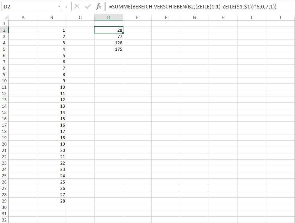
@radial2021 

=SUM(OFFSET(B2,(ROW(1:1)-ROW($1:$1))*6,0,7,1))

Does this formula help? It sums the values from row 2 to row 8 and then from row 9 to row 15 and then row 16 to 22 and so on. I think you can easily adapt it to your sheets if it returns the intended result.

 

[#5]

@OliverScheurich 

This formula works, 

Thank you very much for your help with this, it will save me a lot of time.  

[#6]

@Quadruple_Pawn 

Good Morning,

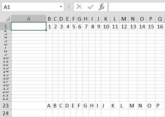
I have another formula problem and I do not know why, see below

I do not see any text issues? the answer I should get is $1,869.14(B23)

Thank you 

[#7]

@radial2021 

=HLOOKUP(B1,'VCM Summary'!B1:BA23,23,FALSE)

=INDEX('VCM Summary'!B23:BA23,MATCH(B1,'VCM Summary'!B1:BA1,0))

XLOOKUP only is available in Office 365 and Excel 2021 and Excel for the web. Which version of Excel do you work with? Alternatives could be HLOOKUP or INDEX and MATCH.

[#8]

I have an earlier version of Excel so the Hlookup worked
Thank you