Formula Troubleshooting

[FHuffman]

I have an excel sheet that contains entries with both "Due" dates and "Completed" dates.  On a separate sheet, I've created a formula that tallies the number of due dates in a specific month and year.

I'm now trying to create another formula that tallies the number of due dates in a specific month and year that are EITHER:

A.  Earlier than the completed date (the entry was overdue when completed)

OR

B.  Earlier than today AND are adjacent to a blank completed date (due date has passed and is still not complete)

I've created a formula that I believe should do just that, but, instead, it's tallying the total number of due dates, regardless of whether or not they were overdue.  Formula is below:

=SUM(IF(ISNUMBER('Simplified Open and Complet'!J:J),IF(YEAR('Simplified Open and Complet'!J:J)=$A$122,IF(MONTH('Simplified Open and Complet'!J:J)=B122,IF(OR('Simplified Open and Complet'!J:J<'Simplified Open and Complet'!K:K,AND('Simplified Open and Complet'!J:J<TODAY(),'Simplified Open and Complet'!K:K="")),1)))))

For context:

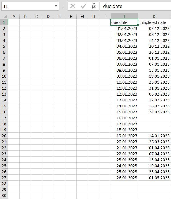
• The J column of the "Simplified Open and Complet" sheet contains due dates.
• The K column contains the completed dates.
• A122 is the year of 2023.
• B122 is the month of January.

The formula should follow the following steps, in order:

1. Check to make sure the due date is not empty
2. Check to make sure the due date is in 2023
3. Check to make sure the due date is in January
4. Check to make sure the due date is EARLIER than the completed date OR (the due date is before today AND the completed date is blank).

If all of the above are true for a given row, the tally should increase by 1.  

I'm sure I'm thinking of something incorrectly in my above formula, but can't figure out where I went wrong. Any help would be appreciated; thank you!

[#2]

I would recommend if you have COUNTIFS to use that:
=COUNTIFS('Simplified Open and Complet'!J:J, "<>",
'Simplified Open and Complet'!J:J, "<"&TODAY(),
'Simplified Open and Complet'!J:J, "<" & 'Simplified Open and Complet'!K:K,
'Simplified Open and Complet'!J:J, ">=" & DATE(A122, B122,1),
'Simplified Open and Complet'!J:J, "<" & EDATE(DATE(A122, B122,1),1) )

[#3]

Hi @mtarler; thanks for the quick response!

When using the above formula, I'm getting a count of 0. The resulting number should be 26, some of which have a blank completed date (K column) and others that have a completed date later than the due date (J column). Only 9 have completed dates that are earlier than the due dates.

[#4 · Accepted solution]

@FHuffman 

=SUM((NOT(ISBLANK('Simplified Open and Complet'!J2:J27)))*(YEAR('Simplified Open and Complet'!J2:J27)=A122)*(MONTH('Simplified Open and Complet'!J2:J27)=B122)*(('Simplified Open and Complet'!J2:J27<'Simplified Open and Complet'!K2:K27)+(('Simplified Open and Complet'!J2:J27<TODAY())*(ISBLANK('Simplified Open and Complet'!K2:K27)))))

An alternative could be this formula. Enter the formula with ctrl+shift+enter if you don't work with Office 365 or Excel 2021.

[#5]

Hi @OliverScheurich,

Thanks for the response!

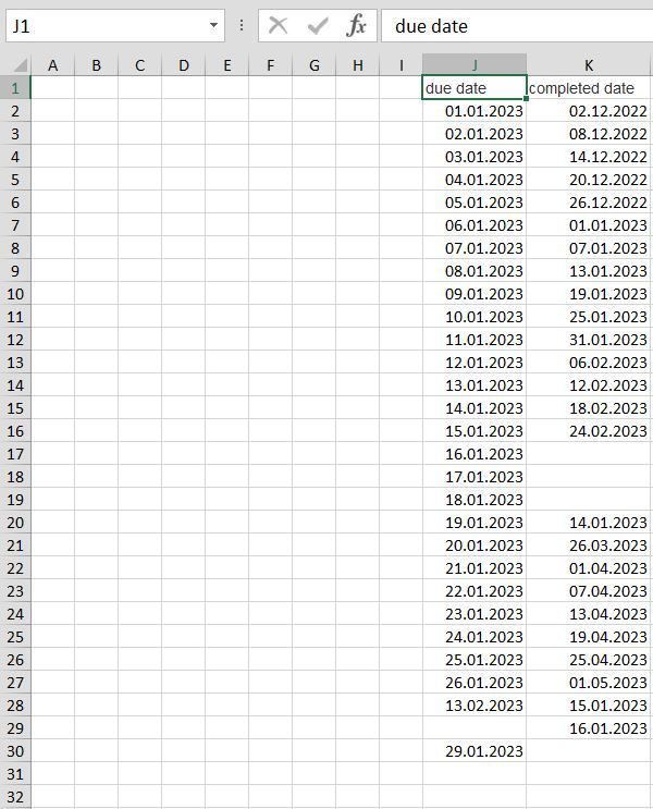
This is almost exactly what I need.  The only problem is that if you expand the ranges to any columns where there is no due date, it no longer works (in your example, if you expand J2:J27 to J2:J28, it gives an error).  Is there something that can be added to ensure that it only considers rows in which the due date contains a value?

[#6]

@FHuffman 

=SUM((NOT(ISBLANK('Simplified Open and Complet'!J2:J1000)))*(YEAR('Simplified Open and Complet'!J2:J1000)=A122)*(MONTH('Simplified Open and Complet'!J2:J1000)=B122)*(('Simplified Open and Complet'!J2:J1000<'Simplified Open and Complet'!K2:K1000)+(('Simplified Open and Complet'!J2:J1000<TODAY())*(ISBLANK('Simplified Open and Complet'!K2:K1000)))))

I've expanded the formula and added entries in sheet "Simplified Open and Complet" and the formula returns the intended result.

[#7]

Hi again @OliverScheurich,

Sorry about that!  It was my mistake.  I was referencing the entire column (J:J and K:K) and the headers of the columns were breaking the formula.  I've changed it now to J2:J$1048576 and K2:K$1048576 and it works like a charm.  I've marked your response as the best answer.

Out of curiosity, is there a more elegant way to do J2:J$1048576 (the entire column minus J1)?  I've noticed that J2:J doesn't work as I'd hoped and was unable to find a better solution.

Thanks again!