Formula Time: tagged as hit or missed

[Julius575]

Hi Excel Community,

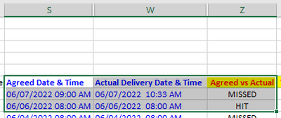
Pls assist formula for column Z. 

this is the scenario:

if column S is more than or late on column W, should be tagged as "missed" in column Z.

if column S is equal or same time or early  to column W, should be tagged as "hit' in column Z.

[#2]

@Julius575 

Attach an Excel file that demonstrates the problem(s).  Click "browse" near the bottom of the reply window.  If you cannot attach a file in this forum, upload it to a file-sharing website and post the download URL here.  I like box.net/files; others like dropbox.com.  You might like onedrive.live.com because it shares the same login as this forum, I believe.

Screen images should include row numbers as well as column names, so that we can refer to them.

The formula in column Z should be of the form

=IF(S2 > W2, "missed", "hit")

In the first row in your screenshot, column Z displays "missed" when you might expect "hit".

My wild guess is:  the "date/time" in column W is text, not numeric time.

Confirm with formulas of the form =ISTEXT(W2).  The format of the cell does not matter; and looks can be deceiving.

For completeness, you should also confirm that the values in column S are indeed numeric.  Confirm with =ISTEXT(S2), which should return FALSE, or with =ISNUMBER(S2).

[#3]

@Joe User 

sharing file for your reference. kindly assist.

[#4]

@Julius575 

First, you have the correct formula in R7 and R8, but not in the rest of column R.

Copy R8 down the entire column through R11853.

-----

Second and most importantly, the data in both column P and Q are text.  As I said, use =ISTEXT(P7) and =ISTEXT(Q7) to confirm.

Ideally, you would convert the data to numeric data/times.  One way that works for me is:

1. Select all the data in column P, starting with P7

2. Click Data > Text To Columns

3. In the first dialog box, select Delimited.  Then click Next

4. In the second dialog box, unselect __all__ delimiters (e.g. Tab by default).  Then click Next

5. In the last dialog box, click Finish

Repeat the same steps with column Q, starting with Q7.

-----

If that does not work for you, the problem might be regional differences.  That is, the form of the dates (and/or times; less likely) on your computer are not m/d/yyyy.

Is that the case?

BTW, __I__ assume the dates are m/d/yyyy.  Could they be d/m/yyyy?

I don't see any dates to disambiguate the two forms.

-----

However, if this will be a recurring problem (that is, you frequently collect new data as text) and you don't want to convert them each time, change the formulas starting in R7 to following form (R7 by example):

=IF(VALUE(P7)>VALUE(Q7),"MISSED","HIT")

(That assumes the form of the dates are consistent with your computer.)

-----

In either case, you have other problems with your data that we can see more clearly with the VALUE formulas, namely:  some rows have empty cells in column Q.  They case #VALUE errors in column R.

You probably need to handle that as a special case in your IF() formula.  But what result do you want in that case?

And less obviously, some rows have just dates in Column P.  In those cases, the time of day is treated as midnight (0:00 AM).  Is that what you want?

Or do you also need to handle that as a special case in your IF() formula?  If so, again, what result do you want in that case?