Formula or function for IF statement based on cell color

[Laurie McDowell]

I don't know how to code in VBA but am trying to automate an if/then calculation based on cell color. As shown in the picture, if the colors of the cells in column B are the same as those in Column G across the row, I want to subtract the values in columns F and K in the same row to return the absolute value of the subtraction in column L. If the colors of the cells are different, I want to add the values in columns F and K and return the value in column L.

I will have multiple tables of varying numbers of rows where I need to perform this operation. Any help is greatly appreciated.

[#2]

@Laurie McDowell 

Hopefully people are still replying to this thread!

I could really do with help here if anyone could help,

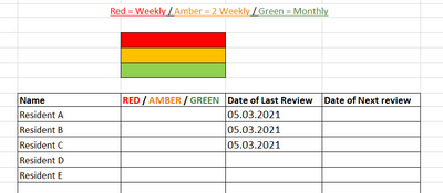
I've been asked to make it so that depending on the colour for the patient, then the date of the next review will auto populate based on the date of the last review. so if Red  would be date of last review plus 7 days, if amber would be last review plus 14 days and if green would be last review plus 1 month. 

I've tried to apply all that is offered in this thread but am well out of my depth!

[#3]

@Kevin Lehrbass 

Hello I have a similar issue.

I have 3 different cells that are colored. Can I create a formula to display a number value in a separate cell based on the colors of those cells.?

If cell B2= color green, then value in cell A2=3.

If cell C2= color green, then value in A2=2.

If cell D2= color green, then value in A2= 1

[#4]

Hi @Dee2021 

For this I think you would need a vba solution.

vba can obtain the background color of a cell and use it in logic (formula or more vba).

Cheers,

Kevin

[#5]

This is long after the fact but @David Rich - it appears your condition for dormant is something like "last 12 months volume is lower than prior year volume"?

If so, you could modify Sergei's formula to:

=IF(C2>0, "Active",IF(B2>C2, "Dormant", "Inactive"))

It also seems like 'Inactive' is specifically a matter of both B2 and C2 being 0? If so:

=IF(C2>0, "Active",IF(B2>C2, "Dormant", (AND(B2=0,C2=0)=TRUE,"Inactive","CHECK")))

This looks for both to be '0' and then returns a CHECK if it ends up that none of the three conditions are met. Say that B2 = C2 and both are greater than 0.

[#6]

@Kevin Lehrbass 

Hi Kevin,
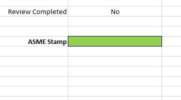
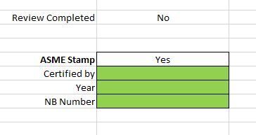
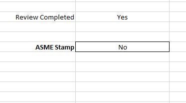
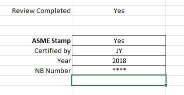
I am looking to use this to look at multiple cells at the same time. I am creating a form that highlights cells based on the information that has been entered. I want a message in the corner stating if the form is completed or not. Because the required information changes I believe the easiest way to accomplish this is to look at all the cells and countif they are green. I have attached some snips of what I am looking for it to do. I am using if statements and formatting to show and hide fields.

[#7]

@Kevin Lehrbass 

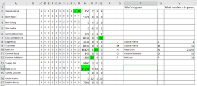
I have a similar need. My spreadsheet is populated each week with new data. Conditional formatting fills the cells in green, that have the highest value in a given column. There is a name in the first column, which needs to be placed in a given cell, when the highest value for that entry is in their row.

I'm trying to come up with a formula or function that can automatically fill in the appropriate answers for columns T and V

[#8]

@CurtRiley 

In V8: =MAX(L2:L17)

In T8: =INDEX(A2:A17, MATCH(V8, L2:L17, 0))

Similar for the others. If you want to be able to fill down:

In V8: =MAX(INDIRECT(U8&"2:"&U8&"17"))

In T8: =INDEX(A$2:A$17, MATCH(V8, INDIRECT(U8&"2:"&U8&"17"), 0))

[#9]

I have a spreadsheet with employees, their name, details and their status (on shift, annual leave etc). Now i need to check in our WFM Software if there have been any new Leave requests and them change the status column for that specific employee, if they have called in sick.

Can someone help me? Paste all entries from WFM (aspect) showing annual leave or sick leave on the side of my spreadsheet. Then I applied conditional formatting so it highlights and employee ID number that is a duplicate (it is on original employee list and also in the leave list from WFM). I now want to use a macro or formula to do something like: if cell is highlighted, then change the status column of that row to the value found in the this same employees status column of the copied WFM table.

Is that possible at all?

[#10]

I am use the colorindex function in several reports, but find that when the colour is changed I have either double click the cell or make a change in the table. Is there anyway way for excel to automatically calculate when cells colours are changed?

[#11]

@Laurie McDowell 

Hello everyone, 

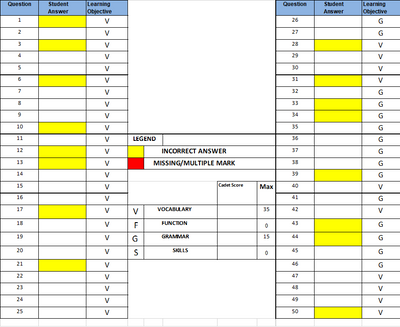
I am new to this feed, so apologies if I am asking for something which has already been answered. I need help with the below, I have tried to break it down so I hope it helps. In a nut shell, I need to put down what the student scored correctly in G19:G23. The yellow color tabs in B3:B27 & K3:K27 reflect what the student answered incorrectly and the white tabs reflect the correct answers. It needs to correspond to the learning objective. As you will notice, it usually changes from "V" to "G" and sometimes we have "F" and "S"

Calculate "Cadet Score" by counting number of correct answered "V"s from column "Learning Objective", which correspond to the non-coloured cells in "Student Answer" column.

Calculate number of correct answered "F"s which correspond with the white coloured cells from the" Student Answer" column

Calculate number of correct answered "G"s from "Learning Objective" column, corresponding with white cells in "Student Answer" column.

Calculate number of correct answered "S"s from "Learning Objective" column which correspond with the non-coloured cells in column "Student Answer".

If there are no "V"s, "F"s, "G"s or "S"s which correspond with white cells in "Student Answer" column, mark "0" under "Cadet Score"

[#12]

why not open a new thread, bro?
And if possible,open full text editor and upload a sample excel.workbook file.
This may explain your problem intuititively。

[#13]

I am not able to upload the excel file,...

[#14]

@Kevin Lehrbass 

Hi Kevin, thank you for your code. It works magic for me. However, can I check if you run into any issue with the file size? I used InteriorColor on an array of 5x80 cells (so 400 executions of the function). The file size changed from 110kb to 45Mb. 

I’m using M365 if it matters. 

Thank you