Formula look at sheet 1, find duplicates in sheet 2 and copy ID from sheet 1 to each duplicate

[Belinea2010]

I am using Excel 2016 and I am in over my head on this.

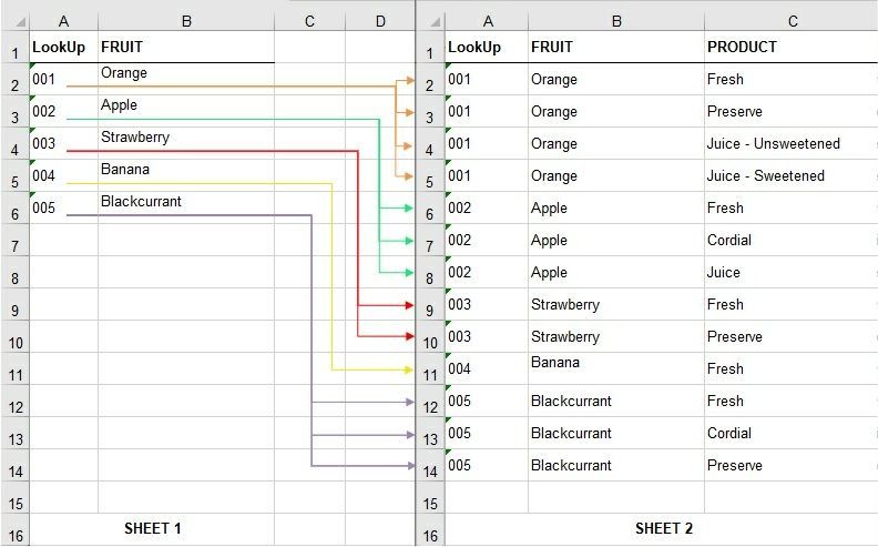
I am trying to write a formula to look at Sheet 1 Column B and for every duplicate in Sheet 2 Column B it will copy the unique anchor/ID Number from Sheet 1 Column A into Sheet 2 Column A as shown by the arrows in the image.

Each worksheet will be updated on a, when needed, basis using a macro to import the Fruit and Product data so the formulas need to be dynamic and able to be copied down each column.

If you look at the example in the image I am using fruit to explain my issue.

For each sheet Row A is the header.

Sheet 1 acts as a master record. Each cell in Column A (LookUp) has a unique number assigned to each type of fruit to act as a anchor/ID Number. Each cell in Column B (Fruit) contains a type of fruit, each entry is unique.

Sheet 2 contains the different types of products made from each fruit. Each cell in Column A (LookUp) will match the equal LookUp in Sheet 1. Each cell in Column B contains the type of fruit. Each cell in Column C contains the type of product made using the fruit. So this means that there will be duplicates of fruit in Column B.

I am trying to write a formula to look at Sheet 1 Column B and for every duplicate in Sheet 2 Column B it will copy the unique anchor/ID Number from Sheet 1 Column A into Sheet 2 Column A as shown by the arrows in the image.

I would really appreciate and help or suggestions.

Thanks in advance.

[#2]

@Belinea2010 Hey you can use Vlookup formula

Try writing this in Sheet 2 Cell B1

=+VLOOKUP(Sheet2!A1,Sheet1!$A$1:$B$100,2,FALSE)

[#3 · Accepted solution]

@Belinea2010 

You may enter into Sheet2!A2

=INDEX(Sheet1!A:A,MATCH(Sheet2!$B2,Sheet1!B:B,0))

and drag it down

[#4]

@DevendraJain 

Hi

Thank you for your suggestion which I really appreciate but as it did not work I thought you might like some feedback.

The formula should go in Sheet 2 Cell A2 and then copied down. It needed to start on row 2 as each sheet has a header row. It goes in Column A because that is where the LookUp needs to be.

Just in case there was a misunderstanding on my part I tried your formula in Sheet 2 Cell A1 and then in Cell B1 but the result was the same. It returns the text of “FRUIT” in the first row and then when copied down it just produces #N/A in each row.

Thanks again

[#5]

@Sergei Baklan 

Hi Sergei

Your formula works perfectly and does exactly what I need.

Thank you so much and I really appreciate your help.

Kind regards Bel

[#6]

@Belinea2010 

Bel, you are welcome, glad to help