formula help - vlookups doing weird stuff

[JMcElwain1]

I know the subject is pretty vague, but I wasn't sure how else to phrase it.

OK, this is going to be a bit longwinded, please ask for clarification if its too messy.

I have a handful of workbooks. The project is to have one main workbook that pulls data from the others. Pretty simple right? The sheets are linked and auto update, that's no problem. The issue arises when I use a vlookup to reference another tab. If the criteria is not found, the cell remains blank due to an IFERROR statement to leave it blank upon error, pretty straightforward.

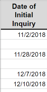
What I want the sheet to do, however, is when the criteria is not found, rather than leave the cell blank, I want the formula to move on to the next cell. One solution I'm finding is to just sort the referenced data. But I don't want to have to do that every time the workbook is opened.

My goal is to have those blank cells replaced with the data found upon matching criteria - make sense?

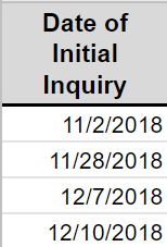
I want the formula to return this:

Thanks for any advice, I'm open to all ideas :)

Jeremy

[#2]

@JMcElwain1 

Which formula you are currently using? Is your formula fetching the values from another Worksheet in the same Workbook? If yes, could you please share a sample workbook (not an image) after removing any sensitive info?

[#3]

@Subodh_Tiwari_sktneer 

Here's what I've got:

Yes, the lookup is fetching values from a tab that holds all of the data. I'm trying to break the data into two tabs based on the vlookup criteria.

I've attached the file. Thank you!

[#4]

@JMcElwain1 

Try this Array Formula which requires confirmation with Ctrl+Shift+Enter instead of Enter alone.

On Booked Sheet,

In A2

=IFERROR(INDEX('All Inquiries'!B$2:B$4,SMALL(IF('All Inquiries'!$A$2:$A$4="B",ROW('All Inquiries'!$A$2:$A$4)-ROW('All Inquiries'!$A$2)+1),ROWS(A$2:A2))),"")

Confirm with Ctrl+Shift+Enter and copy it across and down until you get blank cells.

Exactly same formula you need on Cold Sheet, only the criteria "B" will be replaced with "C" in the formula.

Please find the attached for more details.

If you have access to dynamic array formulas, you may try the Filter function like below...

In A2

=FILTER('All Inquiries'!B2:C4,'All Inquiries'!A2:A4="B","No record found!")

[#5]

@Subodh_Tiwari_sktneer 

Thank you so, so much!

I was able to get the formula working, but I'm still not able to get it to skip rows that don't match the criteria.

Despite being an insider, I don't have access to the FILTER function (yet).

I've attached the updated file for your review, I can't seem to figure out why its not ignoring a row when criteria doesn't match.

Thanks for the help!

Jeremy

[#6]

@JMcElwain1 

That's because you forgot to lock the ranges used in the formula. The correct formula should be like below...

=IFERROR(INDEX('All Inquiries'!B$2:B$4,SMALL(IF('All Inquiries'!$A$2:$A$4="B",ROW('All Inquiries'!$A$2:$A$4)-ROW('All Inquiries'!$A$2)+1),ROWS(A$2:A2))),"")

[#7]

@JMcElwain1 

I prefer this flexible, non-array formula in Booked!A2 of the attached version of your file: 

=IFERROR(INDEX('All Inquiries'!$B$2:$C$4,
AGGREGATE(15,6,(ROW('All Inquiries'!$A$2:$A$4)-1)/('All Inquiries'!$A$2:$A$4="B"),ROW()-1),
MATCH(A$1,'All Inquiries'!$B$1:$C$1,0)),"")